Section MR  Matrix Representations

From A First Course in Linear Algebra
Version 2.20
© 2004.
Licensed under the GNU Free Documentation License.
http://linear.ups.edu/

We have seen that linear transformations whose domain and codomain are vector spaces of columns vectors have a close relationship with matrices (Theorem MBLT, Theorem MLTCV). In this section, we will extend the relationship between matrices and linear transformations to the setting of linear transformations between abstract vector spaces.

Definition MR
Matrix Representation
Suppose that T : U → V is a linear transformation, B = \left \{{u}_{1},\kern 1.95872pt {u}_{2},\kern 1.95872pt {u}_{3},\kern 1.95872pt \mathop{\mathop{…}},\kern 1.95872pt {u}_{n}\right \} is a basis for U of size n, and C is a basis for V of size m. Then the matrix representation of T relative to B and C is the m × n matrix,

{M}_{B,C}^{T } = \left [\left .{ρ}_{ C}\left (T\left ({u}_{1}\right )\right )\right |\left .{ρ}_{C}\left (T\left ({u}_{2}\right )\right )\right |\left .{ρ}_{C}\left (T\left ({u}_{3}\right )\right )\right |\mathop{\mathop{…}}\left |{ρ}_{C}\left (T\left ({u}_{n}\right )\right )\right .\right ]

(This definition contains Notation MR.)

Example OLTTR
One linear transformation, three representations
Consider the linear transformation

S : {P}_{3} → {M}_{22},\quad S\left (a + bx + c{x}^{2} + d{x}^{3}\right ) = \left [\array{ 3a + 7b − 2c − 5d & 8a + 14b − 2c − 11d \cr −4a − 8b + 2c + 6d&12a + 22b − 4c − 17d } \right ]

First, we build a representation relative to the bases,

\eqalignno{ B& = \left \{1 + 2x + {x}^{2} − {x}^{3},\kern 1.95872pt 1 + 3x + {x}^{2} + {x}^{3},\kern 1.95872pt − 1 − 2x + 2{x}^{3},\kern 1.95872pt 2 + 3x + 2{x}^{2} − 5{x}^{3}\right \} & & \cr C & = \left \{\left [\array{ 1&1\cr 1&2 } \right ],\kern 1.95872pt \left [\array{ 2&3\cr 2&5 } \right ],\kern 1.95872pt \left [\array{ −1&−1\cr 0 &−2 } \right ],\kern 1.95872pt \left [\array{ −1&−4\cr −2 &−4 } \right ]\right \}&& }

We evaluate S with each element of the basis for the domain, B, and coordinatize the result relative to the vectors in the basis for the codomain, C.

\eqalignno{ &{ρ}_{C}\left (S\left (1 + 2x + {x}^{2} − {x}^{3}\right )\right ) = {ρ}_{ C}\left (\left [\array{ 20 &45\cr −24 &69 } \right ]\right ) & & \cr &\quad \quad = {ρ}_{C}\left ((−90)\left [\array{ 1&1\cr 1&2 } \right ] + 37\left [\array{ 2&3\cr 2&5 } \right ] + (−40)\left [\array{ −1&−1\cr 0 &−2 } \right ] + 4\left [\array{ −1&−4\cr −2 &−4 } \right ]\right ) = \left [\array{ −90\cr 37 \cr −40\cr 4 } \right ] & & \cr &{ρ}_{C}\left (S\left (1 + 3x + {x}^{2} + {x}^{3}\right )\right ) = {ρ}_{ C}\left (\left [\array{ 17 &37\cr −20 &57 } \right ]\right ) & & \cr &\quad \quad = {ρ}_{C}\left ((−72)\left [\array{ 1&1\cr 1&2 } \right ] + 29\left [\array{ 2&3\cr 2&5 } \right ] + (−34)\left [\array{ −1&−1\cr 0 &−2 } \right ] + 3\left [\array{ −1&−4\cr −2 &−4 } \right ]\right ) = \left [\array{ −72\cr 29 \cr −34\cr 3 } \right ] & & \cr &{ρ}_{C}\left (S\left (−1 − 2x + 2{x}^{3}\right )\right ) = {ρ}_{ C}\left (\left [\array{ −27&−58\cr 32 &−90 } \right ]\right ) & & \cr &\quad \quad = {ρ}_{C}\left (114\left [\array{ 1&1\cr 1&2 } \right ] + (−46)\left [\array{ 2&3\cr 2&5 } \right ] + 54\left [\array{ −1&−1\cr 0 &−2 } \right ] + (−5)\left [\array{ −1&−4\cr −2 &−4 } \right ]\right ) = \left [\array{ 114\cr −46 \cr 54\cr −5 } \right ] & & \cr &{ρ}_{C}\left (S\left (2 + 3x + 2{x}^{2} − 5{x}^{3}\right )\right ) = {ρ}_{ C}\left (\left [\array{ 48 &109\cr −58 &167 } \right ]\right ) & & \cr &\quad \quad = {ρ}_{C}\left ((−220)\left [\array{ 1&1\cr 1&2 } \right ] + 91\left [\array{ 2&3\cr 2&5 } \right ] + −96\left [\array{ −1&−1\cr 0 &−2 } \right ] + 10\left [\array{ −1&−4\cr −2 &−4 } \right ]\right ) = \left [\array{ −220\cr 91 \cr −96\cr 10 } \right ] & & \cr & & }

Thus, employing Definition MR

{ M}_{B,C}^{S} = \left [\array{ −90&−72&114&−220\cr 37 & 29 &−46 & 91 \cr −40&−34& 54 & −96\cr 4 & 3 & −5 & 10 } \right ]

Often we use “nice” bases to build matrix representations and the work involved is much easier. Suppose we take bases

\eqalignno{ D & = \left \{1,\kern 1.95872pt x,\kern 1.95872pt {x}^{2},\kern 1.95872pt {x}^{3}\right \} &E & = \left \{\left [\array{ 1&0 \cr 0&0 } \right ],\kern 1.95872pt \left [\array{ 0&1\cr 0&0 } \right ],\kern 1.95872pt \left [\array{ 0&0\cr 1&0 } \right ],\kern 1.95872pt \left [\array{ 0&0\cr 0&1 } \right ]\right \} & & & & }

The evaluation of S at the elements of D is easy and coordinatization relative to E can be done on sight,

\eqalignno{ {ρ}_{E}\left (S\left (1\right )\right ) & = {ρ}_{E}\left (\left [\array{ 3 & 8\cr −4 &12 } \right ]\right ) & & \cr & = {ρ}_{E}\left (3\left [\array{ 1&0\cr 0&0 } \right ] + 8\left [\array{ 0&1\cr 0&0 } \right ] + (−4)\left [\array{ 0&0\cr 1&0 } \right ] + 12\left [\array{ 0&0\cr 0&1 } \right ]\right ) = \left [\array{ 3\cr 8 \cr −4\cr 12 } \right ] & & \cr {ρ}_{E}\left (S\left (x\right )\right ) & = {ρ}_{E}\left (\left [\array{ 7 &14\cr −8 &22 } \right ]\right ) & & \cr & = {ρ}_{E}\left (7\left [\array{ 1&0\cr 0&0 } \right ] + 14\left [\array{ 0&1\cr 0&0 } \right ] + (−8)\left [\array{ 0&0\cr 1&0 } \right ] + 22\left [\array{ 0&0\cr 0&1 } \right ]\right ) = \left [\array{ 7\cr 14 \cr −8\cr 22 } \right ] & & \cr {ρ}_{E}\left (S\left ({x}^{2}\right )\right ) & = {ρ}_{ E}\left (\left [\array{ −2&−2\cr 2 &−4 } \right ]\right ) & & \cr & = {ρ}_{E}\left ((−2)\left [\array{ 1&0\cr 0&0 } \right ] + (−2)\left [\array{ 0&1\cr 0&0 } \right ] + 2\left [\array{ 0&0\cr 1&0 } \right ] + (−4)\left [\array{ 0&0\cr 0&1 } \right ]\right ) = \left [\array{ −2\cr −2 \cr 2\cr −4 } \right ] & & \cr {ρ}_{E}\left (S\left ({x}^{3}\right )\right ) & = {ρ}_{ E}\left (\left [\array{ −5&−11\cr 6 &−17 } \right ]\right ) & & \cr & = {ρ}_{E}\left ((−5)\left [\array{ 1&0\cr 0&0 } \right ] + (−11)\left [\array{ 0&1\cr 0&0 } \right ] + 6\left [\array{ 0&0\cr 1&0 } \right ] + (−17)\left [\array{ 0&0\cr 0&1 } \right ]\right ) = \left [\array{ −5\cr −11 \cr 6\cr −17 } \right ] & & \cr & & }

So the matrix representation of S relative to D and E is

{ M}_{D,E}^{S} = \left [\array{ 3 & 7 &−2& −5\cr 8 & 14 &−2 &−11 \cr −4&−8& 2 & 6\cr 12 & 22 &−4 &−17 } \right ]

One more time, but now let’s use bases

\eqalignno{ F & = \left \{1 + x − {x}^{2} + 2{x}^{3},\kern 1.95872pt − 1 + 2x + 2{x}^{3},\kern 1.95872pt 2 + x − 2{x}^{2} + 3{x}^{3},\kern 1.95872pt 1 + x + 2{x}^{3}\right \} & & \cr G & = \left \{\left [\array{ 1 &1\cr −1 &2 } \right ],\kern 1.95872pt \left [\array{ −1&2\cr 0 &2 } \right ],\kern 1.95872pt \left [\array{ 2 &1\cr −2 &3 } \right ],\kern 1.95872pt \left [\array{ 1&1\cr 0&2 } \right ]\right \} & & }

and evaluate S with the elements of F, then coordinatize the results relative to G,

\eqalignno{ {ρ}_{G}\left (S\left (1 + x − {x}^{2} + 2{x}^{3}\right )\right ) & = {ρ}_{ G}\left (\left [\array{ 2 &2\cr −2 &4 } \right ]\right ) = {ρ}_{G}\left (2\left [\array{ 1 &1\cr −1 &2 } \right ]\right ) = \left [\array{ 2\cr 0 \cr 0\cr 0 } \right ] & & \cr {ρ}_{G}\left (S\left (−1 + 2x + 2{x}^{3}\right )\right ) & = {ρ}_{ G}\left (\left [\array{ 1&−2\cr 0&−2 } \right ]\right ) = {ρ}_{G}\left ((−1)\left [\array{ −1&2\cr 0 &2 } \right ]\right ) = \left [\array{ 0\cr −1 \cr 0\cr 0 } \right ] & & \cr {ρ}_{G}\left (S\left (2 + x − 2{x}^{2} + 3{x}^{3}\right )\right ) & = {ρ}_{ G}\left (\left [\array{ 2 &1\cr −2 &3 } \right ]\right ) = {ρ}_{G}\left (\left [\array{ 2 &1\cr −2 &3 } \right ]\right ) = \left [\array{ 0\cr 0 \cr 1\cr 0 } \right ] & & \cr {ρ}_{G}\left (S\left (1 + x + 2{x}^{3}\right )\right ) & = {ρ}_{ G}\left (\left [\array{ 0&0\cr 0&0 } \right ]\right ) = {ρ}_{G}\left (0\left [\array{ 1&1\cr 0&2 } \right ]\right ) = \left [\array{ 0\cr 0 \cr 0\cr 0 } \right ] & & \cr & & }

So we arrive at an especially economical matrix representation,

{ M}_{F,G}^{S} = \left [\array{ 2& 0 &0&0\cr 0&−1 &0 &0 \cr 0& 0 &1&0\cr 0& 0 &0 &0 } \right ]

We may choose to use whatever terms we want when we make a definition. Some are arbitrary, while others make sense, but only in light of subsequent theorems. Matrix representation is in the latter category. We begin with a linear transformation and produce a matrix. So what? Here’s the theorem that justifies the term “matrix representation.”

Theorem FTMR
Fundamental Theorem of Matrix Representation
Suppose that T : U → V is a linear transformation, B is a basis for U, C is a basis for V and {M}_{B,C}^{T } is the matrix representation of T relative to B and C. Then, for any u ∈ U,

{ρ}_{C}\left (T\left (u\right )\right ) = {M}_{B,C}^{T }\left ({ρ}_{ B}\left (u\right )\right )

or equivalently

T\left (u\right ) = {ρ}_{C}^{−1}\left ({M}_{ B,C}^{T }\left ({ρ}_{ B}\left (u\right )\right )\right )

Proof   Let B = \left \{{u}_{1},\kern 1.95872pt {u}_{2},\kern 1.95872pt {u}_{3},\kern 1.95872pt \mathop{\mathop{…}},\kern 1.95872pt {u}_{n}\right \} be the basis of U. Since u ∈ U, there are scalars {a}_{1},\kern 1.95872pt {a}_{2},\kern 1.95872pt {a}_{3},\kern 1.95872pt \mathop{\mathop{…}},\kern 1.95872pt {a}_{n} such that

u = {a}_{1}{u}_{1} + {a}_{2}{u}_{2} + {a}_{3}{u}_{3} + \mathrel{⋯} + {a}_{n}{u}_{n}

Then,

\eqalignno{ &{M}_{B,C}^{T }{ρ}_{ B}\left (u\right ) && && \cr & = \left [\left .{ρ}_{C}\left (T\left ({u}_{1}\right )\right )\right |\left .{ρ}_{C}\left (T\left ({u}_{2}\right )\right )\right |\left .{ρ}_{C}\left (T\left ({u}_{3}\right )\right )\right |\mathop{\mathop{…}}\left |{ρ}_{C}\left (T\left ({u}_{n}\right )\right )\right .\right ]{ρ}_{B}\left (u\right ) &&\text{@(a href="#definition.MR")Definition MR@(/a)} &&&& \cr & = \left [\left .{ρ}_{C}\left (T\left ({u}_{1}\right )\right )\right |\left .{ρ}_{C}\left (T\left ({u}_{2}\right )\right )\right |\left .{ρ}_{C}\left (T\left ({u}_{3}\right )\right )\right |\mathop{\mathop{…}}\left |{ρ}_{C}\left (T\left ({u}_{n}\right )\right )\right .\right ]\left [\array{ {a}_{1} \cr {a}_{2} \cr {a}_{3} \cr \mathop{\mathop{⋮}}\cr {a}_{ n} } \right ]&&\text{@(a href="fcla-jsmath-2.20li56.html#definition.VR")Definition VR@(/a)} &&&& \cr & = {a}_{1}{ρ}_{C}\left (T\left ({u}_{1}\right )\right ) + {a}_{2}{ρ}_{C}\left (T\left ({u}_{2}\right )\right ) + \mathrel{⋯} + {a}_{n}{ρ}_{C}\left (T\left ({u}_{n}\right )\right ) &&\text{@(a href="fcla-jsmath-2.20li31.html#definition.MVP")Definition MVP@(/a)}&&&& \cr & = {ρ}_{C}\left ({a}_{1}T\left ({u}_{1}\right ) + {a}_{2}T\left ({u}_{2}\right ) + {a}_{3}T\left ({u}_{3}\right ) + \mathrel{⋯} + {a}_{n}T\left ({u}_{n}\right )\right ) &&\text{@(a href="fcla-jsmath-2.20li51.html#theorem.LTLC")Theorem LTLC@(/a)}&&&& \cr & = {ρ}_{C}\left (T\left ({a}_{1}{u}_{1} + {a}_{2}{u}_{2} + {a}_{3}{u}_{3} + \mathrel{⋯} + {a}_{n}{u}_{n}\right )\right ) &&\text{@(a href="fcla-jsmath-2.20li51.html#theorem.LTLC")Theorem LTLC@(/a)}&&&& \cr & = {ρ}_{C}\left (T\left (u\right )\right ) && && }

The alternative conclusion is obtained as

\eqalignno{ T\left (u\right ) & = {I}_{V }\left (T\left (u\right )\right ) & &\text{@(a href="fcla-jsmath-2.20li54.html#definition.IDLT")Definition IDLT@(/a)} & & & & \cr & = \left ({ρ}_{C}^{−1} ∘ {ρ}_{ C}\right )\left (T\left (u\right )\right ) & &\text{@(a href="fcla-jsmath-2.20li54.html#definition.IVLT")Definition IVLT@(/a)} & & & & \cr & = {ρ}_{C}^{−1}\left ({ρ}_{ C}\left (T\left (u\right )\right )\right ) & &\text{@(a href="fcla-jsmath-2.20li51.html#definition.LTC")Definition LTC@(/a)} & & & & \cr & = {ρ}_{C}^{−1}\left ({M}_{ B,C}^{T }\left ({ρ}_{ B}\left (u\right )\right )\right ) & & & & \cr & & & & }

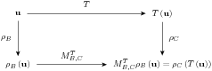
This theorem says that we can apply T to u and coordinatize the result relative to C in V , or we can first coordinatize u relative to B in U, then multiply by the matrix representation. Either way, the result is the same. So the effect of a linear transformation can always be accomplished by a matrix-vector product (Definition MVP). That’s important enough to say again. The effect of a linear transformation is a matrix-vector product.

PIC
Diagram FTMR. Fundamental Theorem of Matrix Representations

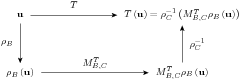
The alternative conclusion of this result might be even more striking. It says that to effect a linear transformation (T) of a vector (u), coordinatize the input (with {ρ}_{B}), do a matrix-vector product (with {M}_{B,C}^{T }), and un-coordinatize the result (with {ρ}_{C}^{−1}). So, absent some bookkeeping about vector representations, a linear transformation is a matrix. To adjust the diagram, we “reverse” the arrow on the right, which means inverting the vector representation {ρ}_{C} on V . Now we can go directly across the top of the diagram, computing the linear transformation between the abstract vector spaces. Or, we can around the other three sides, using vector representation, a matrix-vector product, followed by un-coordinatization.

PIC
Diagram FTMRA. Fundamental Theorem of Matrix Representations (Alternate)

Here’s an example to illustrate how the “action” of a linear transformation can be effected by matrix multiplication.

Example ALTMM
A linear transformation as matrix multiplication
In Example OLTTR we found three representations of the linear transformation S. In this example, we will compute a single output of S in four different ways. First “normally,” then three times over using Theorem FTMR.

Choose p(x) = 3 − x + 2{x}^{2} − 5{x}^{3}, for no particular reason. Then the straightforward application of S to p(x) yields

\eqalignno{ S\left (p(x)\right )& = S\left (3 − x + 2{x}^{2} − 5{x}^{3}\right ) && \cr & = \left [\array{ 3(3) + 7(−1) − 2(2) − 5(−5) & 8(3) + 14(−1) − 2(2) − 11(−5)\cr −4(3) − 8(−1) + 2(2) + 6(−5) &12(3) + 22(−1) − 4(2) − 17(−5) } \right ]&& \cr & = \left [\array{ 23 &61\cr −30 &91 } \right ]&& }

Now use the representation of S relative to the bases B and C and Theorem FTMR. Note that we will employ the following linear combination in moving from the second line to the third,

\eqalignno{ 3 − x + 2{x}^{2} − 5{x}^{3} & = 48(1 + 2x + {x}^{2} − {x}^{3}) + (−20)(1 + 3x + {x}^{2} + {x}^{3})+ & & \cr &\quad \quad (−1)(−1 − 2x + 2{x}^{3}) + (−13)(2 + 3x + 2{x}^{2} − 5{x}^{3}) & & }

\eqalignno{ S\left (p(x)\right ) & = {ρ}_{C}^{−1}\left ({M}_{ B,C}^{S}{ρ}_{ B}\left (p(x)\right )\right ) & & \cr & = {ρ}_{C}^{−1}\left ({M}_{ B,C}^{S}{ρ}_{ B}\left (3 − x + 2{x}^{2} − 5{x}^{3}\right )\right ) & & \cr & = {ρ}_{C}^{−1}\left ({M}_{ B,C}^{S}\left [\array{ 48\cr −20 \cr −1\cr −13 } \right ]\right ) & & \cr & = {ρ}_{C}^{−1}\left (\left [\array{ −90&−72&114&−220\cr 37 & 29 &−46 & 91 \cr −40&−34& 54 & −96\cr 4 & 3 & −5 & 10 } \right ]\left [\array{ 48\cr −20 \cr −1\cr −13 } \right ]\right ) & & \cr & = {ρ}_{C}^{−1}\left (\left [\array{ −134\cr 59 \cr −46\cr 7 } \right ]\right ) & & \cr & = (−134)\left [\array{ 1&1\cr 1&2 } \right ] + 59\left [\array{ 2&3\cr 2&5 } \right ] + (−46)\left [\array{ −1&−1\cr 0 &−2 } \right ] + 7\left [\array{ −1&−4\cr −2 &−4 } \right ] & & \cr & = \left [\array{ 23 &61\cr −30 &91 } \right ] & & }
Again, but now with “nice” bases like D and E, and the computations are more transparent.
\eqalignno{ S\left (p(x)\right ) & = {ρ}_{E}^{−1}\left ({M}_{ D,E}^{S}{ρ}_{ D}\left (p(x)\right )\right ) & & \cr & = {ρ}_{E}^{−1}\left ({M}_{ D,E}^{S}{ρ}_{ D}\left (3 − x + 2{x}^{2} − 5{x}^{3}\right )\right ) & & \cr & = {ρ}_{E}^{−1}\left ({M}_{ D,E}^{S}{ρ}_{ D}\left (3(1) + (−1)(x) + 2({x}^{2}) + (−5)({x}^{3})\right )\right ) & & \cr & = {ρ}_{E}^{−1}\left ({M}_{ D,E}^{S}\left [\array{ 3\cr −1 \cr 2\cr −5 } \right ]\right ) & & \cr & = {ρ}_{E}^{−1}\left (\left [\array{ 3 & 7 &−2& −5\cr 8 & 14 &−2 &−11 \cr −4&−8& 2 & 6\cr 12 & 22 &−4 &−17 } \right ]\left [\array{ 3\cr −1 \cr 2\cr −5 } \right ]\right ) & & \cr & = {ρ}_{E}^{−1}\left (\left [\array{ 23\cr 61 \cr −30\cr 91 } \right ]\right ) & & \cr & = 23\left [\array{ 1&0\cr 0&0 } \right ] + 61\left [\array{ 0&1\cr 0&0 } \right ] + (−30)\left [\array{ 0&0\cr 1&0 } \right ] + 91\left [\array{ 0&0\cr 0&1 } \right ] & & \cr & = \left [\array{ 23 &61\cr −30 &91 } \right ] & & }

OK, last time, now with the bases F and G. The coordinatizations will take some work this time, but the matrix-vector product (Definition MVP) (which is the actual action of the linear transformation) will be especially easy, given the diagonal nature of the matrix representation, {M}_{F,G}^{S}. Here we go,

\eqalignno{ S\left (p(x)\right )& = {ρ}_{G}^{−1}\left ({M}_{ F,G}^{S}{ρ}_{ F }\left (p(x)\right )\right ) && \cr & = {ρ}_{G}^{−1}\left ({M}_{ F,G}^{S}{ρ}_{ F }\left (3 − x + 2{x}^{2} − 5{x}^{3}\right )\right ) && \cr & = {ρ}_{G}^{−1}\left ({M}_{ F,G}^{S}{ρ}_{ F }\left (32(1 + x − {x}^{2} + 2{x}^{3}) − 7(−1 + 2x + 2{x}^{3}) − 17(2 + x − 2{x}^{2} + 3{x}^{3}) − 2(1 + x + 2{x}^{3})\right )\right ) && \cr & = {ρ}_{G}^{−1}\left ({M}_{ F,G}^{S}\left [\array{ 32\cr −7 \cr −17\cr −2 } \right ]\right ) && \cr & = {ρ}_{G}^{−1}\left (\left [\array{ 2& 0 &0&0\cr 0&−1 &0 &0 \cr 0& 0 &1&0\cr 0& 0 &0 &0 } \right ]\left [\array{ 32\cr −7 \cr −17\cr −2 } \right ]\right ) && \cr & = {ρ}_{G}^{−1}\left (\left [\array{ 64\cr 7 \cr −17\cr 0 } \right ]\right ) && \cr & = 64\left [\array{ 1 &1\cr −1 &2 } \right ] + 7\left [\array{ −1&2\cr 0 &2 } \right ] + (−17)\left [\array{ 2 &1\cr −2 &3 } \right ] + 0\left [\array{ 1&1\cr 0&2 } \right ]&& \cr & = \left [\array{ 23 &61\cr −30 &91 } \right ] && }

This example is not meant to necessarily illustrate that any one of these four computations is simpler than the others. Instead, it is meant to illustrate the many different ways we can arrive at the same result, with the last three all employing a matrix representation to effect the linear transformation.

We will use Theorem FTMR frequently in the next few sections. A typical application will feel like the linear transformation T “commutes” with a vector representation, {ρ}_{C}, and as it does the transformation morphs into a matrix, {M}_{B,C}^{T }, while the vector representation changes to a new basis, {ρ}_{B}. Or vice-versa.

Subsection NRFO: New Representations from Old

In Subsection LT.NLTFO we built new linear transformations from other linear transformations. Sums, scalar multiples and compositions. These new linear transformations will have matrix representations as well. How do the new matrix representations relate to the old matrix representations? Here are the three theorems.

Theorem MRSLT
Matrix Representation of a Sum of Linear Transformations
Suppose that T : U → V and S : U → V are linear transformations, B is a basis of U and C is a basis of V . Then

{M}_{B,C}^{T+S} = {M}_{ B,C}^{T } + {M}_{ B,C}^{S}

Proof   Let x be any vector in {ℂ}^{n}. Define u ∈ U by u = {ρ}_{B}^{−1}\left (x\right ), so x = {ρ}_{B}\left (u\right ). Then,

\eqalignno{ {M}_{B,C}^{T+S}x & = {M}_{ B,C}^{T+S}{ρ}_{ B}\left (u\right ) & &\text{Substitution} & & & & \cr & = {ρ}_{C}\left (\left (T + S\right )\left (u\right )\right ) & &\text{@(a href="#theorem.FTMR")Theorem FTMR@(/a)} & & & & \cr & = {ρ}_{C}\left (T\left (u\right ) + S\left (u\right )\right ) & &\text{@(a href="fcla-jsmath-2.20li51.html#definition.LTA")Definition LTA@(/a)} & & & & \cr & = {ρ}_{C}\left (T\left (u\right )\right ) + {ρ}_{C}\left (S\left (u\right )\right ) & &\text{@(a href="fcla-jsmath-2.20li51.html#definition.LT")Definition LT@(/a)} & & & & \cr & = {M}_{B,C}^{T }\left ({ρ}_{ B}\left (u\right )\right ) + {M}_{B,C}^{S}\left ({ρ}_{ B}\left (u\right )\right ) & &\text{@(a href="#theorem.FTMR")Theorem FTMR@(/a)} & & & & \cr & = \left ({M}_{B,C}^{T } + {M}_{ B,C}^{S}\right ){ρ}_{ B}\left (u\right ) & &\text{@(a href="fcla-jsmath-2.20li31.html#theorem.MMDAA")Theorem MMDAA@(/a)} & & & & \cr & = \left ({M}_{B,C}^{T } + {M}_{ B,C}^{S}\right )x & &\text{Substitution} & & & & }

Since the matrices {M}_{B,C}^{T+S} and {M}_{B,C}^{T } + {M}_{ B,C}^{S} have equal matrix-vector products for every vector in {ℂ}^{n}, by Theorem EMMVP they are equal matrices. (Now would be a good time to double-back and study the proof of Theorem EMMVP. You did promise to come back to this theorem sometime, didn’t you?)

Theorem MRMLT
Matrix Representation of a Multiple of a Linear Transformation
Suppose that T : U → V is a linear transformation, α ∈ {ℂ}^{}, B is a basis of U and C is a basis of V . Then

{M}_{B,C}^{αT } = α{M}_{ B,C}^{T }

Proof   Let x be any vector in {ℂ}^{n}. Define u ∈ U by u = {ρ}_{B}^{−1}\left (x\right ), so x = {ρ}_{B}\left (u\right ). Then,

\eqalignno{ {M}_{B,C}^{αT }x & = {M}_{ B,C}^{αT }{ρ}_{ B}\left (u\right ) & &\text{Substitution} & & & & \cr & = {ρ}_{C}\left (\left (αT\right )\left (u\right )\right ) & &\text{@(a href="#theorem.FTMR")Theorem FTMR@(/a)} & & & & \cr & = {ρ}_{C}\left (αT\left (u\right )\right ) & &\text{@(a href="fcla-jsmath-2.20li51.html#definition.LTSM")Definition LTSM@(/a)} & & & & \cr & = α{ρ}_{C}\left (T\left (u\right )\right ) & &\text{@(a href="fcla-jsmath-2.20li51.html#definition.LT")Definition LT@(/a)} & & & & \cr & = α\left ({M}_{B,C}^{T }{ρ}_{ B}\left (u\right )\right ) & &\text{@(a href="#theorem.FTMR")Theorem FTMR@(/a)} & & & & \cr & = \left (α{M}_{B,C}^{T }\right ){ρ}_{ B}\left (u\right ) & &\text{@(a href="fcla-jsmath-2.20li31.html#theorem.MMSMM")Theorem MMSMM@(/a)} & & & & \cr & = \left (α{M}_{B,C}^{T }\right )x & &\text{Substitution} & & & & }

Since the matrices {M}_{B,C}^{αT } and α{M}_{B,C}^{T } have equal matrix-vector products for every vector in {ℂ}^{n}, by Theorem EMMVP they are equal matrices.

The vector space of all linear transformations from U to V is now isomorphic to the vector space of all m × n matrices.

Theorem MRCLT
Matrix Representation of a Composition of Linear Transformations
Suppose that T : U → V and S : V → W are linear transformations, B is a basis of U, C is a basis of V , and D is a basis of W. Then

{M}_{B,D}^{S∘T } = {M}_{ C,D}^{S}{M}_{ B,C}^{T }

Proof   Let x be any vector in {ℂ}^{n}. Define u ∈ U by u = {ρ}_{B}^{−1}\left (x\right ), so x = {ρ}_{B}\left (u\right ). Then,

\eqalignno{ {M}_{B,D}^{S∘T }x & = {M}_{ B,D}^{S∘T }{ρ}_{ B}\left (u\right ) & &\text{Substitution} & & & & \cr & = {ρ}_{D}\left (\left (S ∘ T\right )\left (u\right )\right ) & &\text{@(a href="#theorem.FTMR")Theorem FTMR@(/a)} & & & & \cr & = {ρ}_{D}\left (S\left (T\left (u\right )\right )\right ) & &\text{@(a href="fcla-jsmath-2.20li51.html#definition.LTC")Definition LTC@(/a)} & & & & \cr & = {M}_{C,D}^{S}{ρ}_{ C}\left (T\left (u\right )\right ) & &\text{@(a href="#theorem.FTMR")Theorem FTMR@(/a)} & & & & \cr & = {M}_{C,D}^{S}\left ({M}_{ B,C}^{T }{ρ}_{ B}\left (u\right )\right ) & &\text{@(a href="#theorem.FTMR")Theorem FTMR@(/a)} & & & & \cr & = \left ({M}_{C,D}^{S}{M}_{ B,C}^{T }\right ){ρ}_{ B}\left (u\right ) & &\text{@(a href="fcla-jsmath-2.20li31.html#theorem.MMA")Theorem MMA@(/a)} & & & & \cr & = \left ({M}_{C,D}^{S}{M}_{ B,C}^{T }\right )x & &\text{Substitution} & & & & }

Since the matrices {M}_{B,D}^{S∘T } and {M}_{C,D}^{S}{M}_{ B,C}^{T } have equal matrix-vector products for every vector in {ℂ}^{n}, by Theorem EMMVP they are equal matrices.

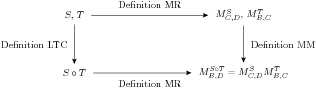
This is the second great surprise of introductory linear algebra. Matrices are linear transformations (functions, really), and matrix multiplication is function composition! We can form the composition of two linear transformations, then form the matrix representation of the result. Or we can form the matrix representation of each linear transformation separately, then multiply the two representations together via Definition MM. In either case, we arrive at the same result.

Example MPMR
Matrix product of matrix representations
Consider the two linear transformations,

\eqalignno{ T : {ℂ}^{2} → {P}_{ 2} &\quad T\left (\left [\array{ a\cr b } \right ]\right ) = (−a + 3b) + (2a + 4b)x + (a − 2b){x}^{2} & & \cr S : {P}_{2} → {M}_{22} &\quad \ S\left (a + bx + c{x}^{2}\right ) = \left [\array{ 2a + b + 2c& a + 4b − c \cr −a + 3c &3a + b + 2c } \right ] & & }

and bases for {ℂ}^{2}, {P}_{2} and {M}_{22} (respectively),

\eqalignno{ B & = \left \{\left [\array{ 3\cr 1 } \right ],\kern 1.95872pt \left [\array{ 2\cr 1 } \right ]\right \} & & \cr C & = \left \{1 − 2x + {x}^{2},\kern 1.95872pt − 1 + 3x,\kern 1.95872pt 2x + 3{x}^{2}\right \} & & \cr D & = \left \{\left [\array{ 1&−2\cr 1&−1 } \right ],\kern 1.95872pt \left [\array{ 1&−1\cr 1& 2 } \right ],\kern 1.95872pt \left [\array{ −1&2\cr 0 &0 } \right ],\kern 1.95872pt \left [\array{ 2&−3\cr 2& 2 } \right ]\right \} & & }

Begin by computing the new linear transformation that is the composition of T and S (Definition LTC, Theorem CLTLT), \left (S ∘ T\right ): {ℂ}^{2} → {M}_{ 22},

\eqalignno{ \left (S ∘ T\right )\left (\left [\array{ a\cr b } \right ]\right )& = S\left (T\left (\left [\array{ a\cr b } \right ]\right )\right )&& \cr & = S\left ((−a + 3b) + (2a + 4b)x + (a − 2b){x}^{2}\right ) && \cr & = \left [\array{ 2(−a + 3b) + (2a + 4b) + 2(a − 2b)& (−a + 3b) + 4(2a + 4b) − (a − 2b)\cr −(−a + 3b) + 3(a − 2b) &3(−a + 3b) + (2a + 4b) + 2(a − 2b) } \right ] && \cr & = \left [\array{ 2a + 6b&6a + 21b\cr 4a − 9b & a + 9b } \right ] && }

Now compute the matrix representations (Definition MR) for each of these three linear transformations (T, S, S ∘ T), relative to the appropriate bases. First for T,

\eqalignno{ {ρ}_{C}\left (T\left (\left [\array{ 3\cr 1 } \right ]\right )\right )& = {ρ}_{C}\left (10x + {x}^{2}\right ) && \cr & = {ρ}_{C}\left (28(1 − 2x + {x}^{2}) + 28(−1 + 3x) + (−9)(2x + 3{x}^{2})\right ) = \left [\array{ 28\cr 28 \cr −9 } \right ] && \cr {ρ}_{C}\left (T\left (\left [\array{ 2\cr 1 } \right ]\right )\right )& = {ρ}_{C}\left (1 + 8x\right ) && \cr & = {ρ}_{C}\left (33(1 − 2x + {x}^{2}) + 32(−1 + 3x) + (−11)(2x + 3{x}^{2})\right ) = \left [\array{ 33\cr 32 \cr −11 } \right ]&& \cr & & }

So we have the matrix representation of T,

{ M}_{B,C}^{T } = \left [\array{ 28& 33\cr 28 & 32 \cr −9&−11 } \right ]

Now, a representation of S,

\eqalignno{ {ρ}_{D}\left (S\left (1 − 2x + {x}^{2}\right )\right )& = {ρ}_{ D}\left (\left [\array{ 2&−8\cr 2& 3 } \right ]\right ) && \cr & = {ρ}_{D}\left ((−11)\left [\array{ 1&−2\cr 1&−1 } \right ] + (−21)\left [\array{ 1&−1\cr 1& 2 } \right ] + 0\left [\array{ −1&2\cr 0 &0 } \right ] + (17)\left [\array{ 2&−3\cr 2& 2 } \right ]\right )&& \cr & = \left [\array{ −11\cr −21 \cr 0\cr 17} \right ] && \cr {ρ}_{D}\left (S\left (−1 + 3x\right )\right ) & = {ρ}_{D}\left (\left [\array{ 1&11\cr 1& 0} \right ]\right ) && \cr & = {ρ}_{D}\left (26\left [\array{ 1&−2\cr 1&−1 } \right ] + 51\left [\array{ 1&−1\cr 1& 2 } \right ] + 0\left [\array{ −1&2\cr 0 &0 } \right ] + (−38)\left [\array{ 2&−3\cr 2& 2 } \right ]\right ) && \cr & = \left [\array{ 26\cr 51 \cr 0\cr −38 } \right ] && \cr {ρ}_{D}\left (S\left (2x + 3{x}^{2}\right )\right ) & = {ρ}_{ D}\left (\left [\array{ 8&5\cr 9&8 } \right ]\right ) && \cr & = {ρ}_{D}\left (34\left [\array{ 1&−2\cr 1&−1 } \right ] + 67\left [\array{ 1&−1\cr 1& 2 } \right ] + 1\left [\array{ −1&2\cr 0 &0 } \right ] + (−46)\left [\array{ 2&−3\cr 2& 2 } \right ]\right ) && \cr & = \left [\array{ 34\cr 67 \cr 1\cr −46 } \right ] && \cr & & }

So we have the matrix representation of S,

{ M}_{C,D}^{S} = \left [\array{ −11& 26 & 34\cr −21 & 51 & 67 \cr 0 & 0 & 1\cr 17 &−38 &−46 } \right ]

Finally, a representation of S ∘ T,

\eqalignno{ {ρ}_{D}\left (\left (S ∘ T\right )\left (\left [\array{ 3\cr 1 } \right ]\right )\right )& = {ρ}_{D}\left (\left [\array{ 12&39\cr 3 &12 } \right ]\right ) && \cr & = {ρ}_{D}\left (114\left [\array{ 1&−2\cr 1&−1 } \right ] + 237\left [\array{ 1&−1\cr 1& 2 } \right ] + (−9)\left [\array{ −1&2\cr 0 &0 } \right ] + (−174)\left [\array{ 2&−3\cr 2& 2 } \right ]\right )&& \cr & = \left [\array{ 114\cr 237 \cr −9\cr −174 } \right ] && \cr {ρ}_{D}\left (\left (S ∘ T\right )\left (\left [\array{ 2\cr 1 } \right ]\right )\right )& = {ρ}_{D}\left (\left [\array{ 10&33\cr −1 &11 } \right ]\right ) && \cr & = {ρ}_{D}\left (95\left [\array{ 1&−2\cr 1&−1 } \right ] + 202\left [\array{ 1&−1\cr 1& 2 } \right ] + (−11)\left [\array{ −1&2\cr 0 &0 } \right ] + (−149)\left [\array{ 2&−3\cr 2& 2 } \right ]\right )&& \cr & = \left [\array{ 95\cr 202 \cr −11\cr −149 } \right ] && \cr & & }

So we have the matrix representation of S ∘ T,

{ M}_{B,D}^{S∘T } = \left [\array{ 114 & 95\cr 237 & 202 \cr −9 & −11\cr −174 &−149 } \right ]

Now, we are all set to verify the conclusion of Theorem MRCLT,

\eqalignno{ {M}_{C,D}^{S}{M}_{ B,C}^{T } & = \left [\array{ −11& 26 & 34\cr −21 & 51 & 67 \cr 0 & 0 & 1\cr 17 &−38 &−46 } \right ]\left [\array{ 28& 33\cr 28 & 32 \cr −9&−11 } \right ] & & \cr & = \left [\array{ 114 & 95\cr 237 & 202 \cr −9 & −11\cr −174 &−149 } \right ] & & \cr & = {M}_{B,D}^{S∘T } & & }

We have intentionally used non-standard bases. If you were to choose “nice” bases for the three vector spaces, then the result of the theorem might be rather transparent. But this would still be a worthwhile exercise — give it a go.

A diagram, similar to ones we have seen earlier, might make the importance of this theorem clearer,

PIC
Diagram MRCLT. Matrix Representation and Composition of Linear Transformations

One of our goals in the first part of this book is to make the definition of matrix multiplication (Definition MVP, Definition MM) seem as natural as possible. However, many are brought up with an entry-by-entry description of matrix multiplication (Theorem ME) as the definition of matrix multiplication, and then theorems about columns of matrices and linear combinations follow from that definition. With this unmotivated definition, the realization that matrix multiplication is function composition is quite remarkable. It is an interesting exercise to begin with the question, “What is the matrix representation of the composition of two linear transformations?” and then, without using any theorems about matrix multiplication, finally arrive at the entry-by-entry description of matrix multiplication. Try it yourself (Exercise MR.T80).

Subsection PMR: Properties of Matrix Representations

It will not be a surprise to discover that the kernel and range of a linear transformation are closely related to the null space and column space of the transformation’s matrix representation. Perhaps this idea has been bouncing around in your head already, even before seeing the definition of a matrix representation. However, with a formal definition of a matrix representation (Definition MR), and a fundamental theorem to go with it (Theorem FTMR) we can be formal about the relationship, using the idea of isomorphic vector spaces (Definition IVS). Here are the twin theorems.

Theorem KNSI
Kernel and Null Space Isomorphism
Suppose that T : U → V is a linear transformation, B is a basis for U of size n, and C is a basis for V . Then the kernel of T is isomorphic to the null space of {M}_{B,C}^{T },

K\kern -1.95872pt \left (T\right )\mathop{\mathop{≅}}N\kern -1.95872pt \left ({M}_{B,C}^{T }\right )

Proof   To establish that two vector spaces are isomorphic, we must find an isomorphism between them, an invertible linear transformation (Definition IVS). The kernel of the linear transformation T, K\kern -1.95872pt \left (T\right ), is a subspace of U, while the null space of the matrix representation, N\kern -1.95872pt \left ({M}_{B,C}^{T }\right ) is a subspace of {ℂ}^{n}. The function {ρ}_{B} is defined as a function from U to {ℂ}^{n}, but we can just as well employ the definition of {ρ}_{B} as a function from K\kern -1.95872pt \left (T\right ) to N\kern -1.95872pt \left ({M}_{B,C}^{T }\right ).

We must first insure that if we choose an input for {ρ}_{B} from K\kern -1.95872pt \left (T\right ) that then the output will be an element of N\kern -1.95872pt \left ({M}_{B,C}^{T }\right ). So suppose that u ∈K\kern -1.95872pt \left (T\right ). Then

\eqalignno{ {M}_{B,C}^{T }{ρ}_{ B}\left (u\right ) & = {ρ}_{C}\left (T\left (u\right )\right ) & &\text{@(a href="#theorem.FTMR")Theorem FTMR@(/a)} & & & & \cr & = {ρ}_{C}\left (0\right ) & &\text{@(a href="fcla-jsmath-2.20li52.html#definition.KLT")Definition KLT@(/a)} & & & & \cr & = 0 & &\text{@(a href="fcla-jsmath-2.20li51.html#theorem.LTTZZ")Theorem LTTZZ@(/a)} & & & & \cr & & & & }

This says that {ρ}_{B}\left (u\right ) ∈N\kern -1.95872pt \left ({M}_{B,C}^{T }\right ), as desired.

The restriction in the size of the domain and codomain {ρ}_{B} will not affect the fact that {ρ}_{B} is a linear transformation (Theorem VRLT), nor will it affect the fact that {ρ}_{B} is injective (Theorem VRI). Something must be done though to verify that {ρ}_{B} is surjective. To this end, appeal to the definition of surjective (Definition SLT), and suppose that we have an element of the codomain, x ∈N\kern -1.95872pt \left ({M}_{B,C}^{T }\right ) ⊆ {ℂ}^{n} and we wish to find an element of the domain with x as its image. We now show that the desired element of the domain is u = {ρ}_{B}^{−1}\left (x\right ). First, verify that u ∈K\kern -1.95872pt \left (T\right ),

\eqalignno{ T\left (u\right ) & = T\left ({ρ}_{B}^{−1}\left (x\right )\right ) & & & & \cr & = {ρ}_{C}^{−1}\left ({M}_{ B,C}^{T }\left ({ρ}_{ B}\left ({ρ}_{B}^{−1}\left (x\right )\right )\right )\right ) & &\text{@(a href="#theorem.FTMR")Theorem FTMR@(/a)} & & & & \cr & = {ρ}_{C}^{−1}\left ({M}_{ B,C}^{T }\left ({I}_{{ ℂ}^{n}}\left (x\right )\right )\right ) & &\text{@(a href="fcla-jsmath-2.20li54.html#definition.IVLT")Definition IVLT@(/a)} & & & & \cr & = {ρ}_{C}^{−1}\left ({M}_{ B,C}^{T }x\right ) & &\text{@(a href="fcla-jsmath-2.20li54.html#definition.IDLT")Definition IDLT@(/a)} & & & & \cr & = {ρ}_{C}^{−1}\left ({0}_{{ ℂ}^{n}}\right ) & &\text{@(a href="fcla-jsmath-2.20li52.html#definition.KLT")Definition KLT@(/a)} & & & & \cr & = {0}_{V } & &\text{@(a href="fcla-jsmath-2.20li51.html#theorem.LTTZZ")Theorem LTTZZ@(/a)} & & & & \text{Second, verify that the proposed isomorphism, ${ρ}_{B}$, takes $u$ to $x$,} \cr {ρ}_{B}\left (u\right ) & = {ρ}_{B}\left ({ρ}_{B}^{−1}\left (x\right )\right ) & &\text{Substitution} & & & & \cr & = {I}_{{ℂ}^{n}}\left (x\right ) & &\text{@(a href="fcla-jsmath-2.20li54.html#definition.IVLT")Definition IVLT@(/a)} & & & & \cr & = x & &\text{@(a href="fcla-jsmath-2.20li54.html#definition.IDLT")Definition IDLT@(/a)} & & & &

}

With {ρ}_{B} demonstrated to be an injective and surjective linear transformation from K\kern -1.95872pt \left (T\right ) to N\kern -1.95872pt \left ({M}_{B,C}^{T }\right ), Theorem ILTIS tells us {ρ}_{B} is invertible, and so by Definition IVS, we say K\kern -1.95872pt \left (T\right ) and N\kern -1.95872pt \left ({M}_{B,C}^{T }\right ) are isomorphic.

Example KVMR
Kernel via matrix representation
Consider the kernel of the linear transformation

T : {M}_{22} → {P}_{2},\quad T\left (\left [\array{ a&b\cr c&d } \right ]\right ) = (2a−b+c−5d)+(a+4b+5b+2d)x+(3a−2b+c−8d){x}^{2}

We will begin with a matrix representation of T relative to the bases for {M}_{22} and {P}_{2} (respectively),

\eqalignno{ B & = \left \{\left [\array{ 1 & 2\cr −1 &−1 } \right ],\kern 1.95872pt \left [\array{ 1 & 3\cr −1 &−4 } \right ],\kern 1.95872pt \left [\array{ 1& 2\cr 0&−2 } \right ],\kern 1.95872pt \left [\array{ 2 & 5\cr −2 &−4 } \right ]\right \} & & \cr C & = \left \{1 + x + {x}^{2},\kern 1.95872pt 2 + 3x,\kern 1.95872pt − 1 − 2{x}^{2}\right \} & & }

Then,

\eqalignno{ {ρ}_{C}\left (T\left (\left [\array{ 1 & 2\cr −1 &−1 } \right ]\right )\right ) & = {ρ}_{C}\left (4 + 2x + 6{x}^{2}\right ) & & \cr & = {ρ}_{C}\left (2(1 + x + {x}^{2}) + 0(2 + 3x) + (−2)(−1 − 2{x}^{2})\right ) & & \cr & = \left [\array{ 2\cr 0 \cr −2 } \right ] & & \cr {ρ}_{C}\left (T\left (\left [\array{ 1 & 3\cr −1 &−4 } \right ]\right )\right ) & = {ρ}_{C}\left (18 + 28{x}^{2}\right ) & & \cr & = {ρ}_{C}\left ((−24)(1 + x + {x}^{2}) + 8(2 + 3x) + (−26)(−1 − 2{x}^{2})\right ) & & \cr & = \left [\array{ −24\cr 8 \cr −26 } \right ] & & \cr {ρ}_{C}\left (T\left (\left [\array{ 1& 2\cr 0&−2 } \right ]\right )\right ) & = {ρ}_{C}\left (10 + 5x + 15{x}^{2}\right ) & & \cr & = {ρ}_{C}\left (5(1 + x + {x}^{2}) + 0(2 + 3x) + (−5)(−1 − 2{x}^{2})\right ) & & \cr & = \left [\array{ 5\cr 0 \cr −5 } \right ] & & \cr {ρ}_{C}\left (T\left (\left [\array{ 2 & 5\cr −2 &−4 } \right ]\right )\right ) & = {ρ}_{C}\left (17 + 4x + 26{x}^{2}\right ) & & \cr & = {ρ}_{C}\left ((−8)(1 + x + {x}^{2}) + (4)(2 + 3x) + (−17)(−1 − 2{x}^{2})\right ) & & \cr & = \left [\array{ −8\cr 4 \cr −17 } \right ] & & }

So the matrix representation of T (relative to B and C) is

{ M}_{B,C}^{T } = \left [\array{ 2 &−24& 5 & −8\cr 0 & 8 & 0 & 4 \cr −2&−26&−5&−17 } \right ]

We know from Theorem KNSI that the kernel of the linear transformation T is isomorphic to the null space of the matrix representation {M}_{B,C}^{T } and by studying the proof of Theorem KNSI we learn that {ρ}_{B} is an isomorphism between these null spaces. Rather than trying to compute the kernel of T using definitions and techniques from Chapter LT we will instead analyze the null space of {M}_{B,C}^{T } using techniques from way back in Chapter V. First row-reduce {M}_{B,C}^{T },

\left [\array{ 2 &−24& 5 & −8\cr 0 & 8 & 0 & 4 \cr −2&−26&−5&−17 } \right ]\mathop{\longrightarrow}\limits_{}^{\text{RREF}}\left [\array{ \text{1}&0&{5\over 2}&2 \cr 0&\text{1}&0&{1\over 2} \cr 0&0&0&0 } \right ]

So, by Theorem BNS, a basis for N\kern -1.95872pt \left ({M}_{B,C}^{T }\right ) is

\left \langle \left \{\left [\array{ −{5\over 2} \cr 0\cr 1 \cr 0 } \right ],\kern 1.95872pt \left [\array{ −2 \cr −{1\over 2} \cr 0\cr 1 } \right ]\right \}\right \rangle

We can now convert this basis of N\kern -1.95872pt \left ({M}_{B,C}^{T }\right ) into a basis of K\kern -1.95872pt \left (T\right ) by applying {ρ}_{B}^{−1} to each element of the basis,

\eqalignno{ {ρ}_{B}^{−1}\left (\left [\array{ −{5\over 2} \cr 0\cr 1 \cr 0 } \right ]\right ) & = (−{5\over 2})\left [\array{ 1 & 2\cr −1 &−1 } \right ] + 0\left [\array{ 1 & 3\cr −1 &−4 } \right ] + 1\left [\array{ 1& 2\cr 0&−2 } \right ] + 0\left [\array{ 2 & 5\cr −2 &−4 } \right ] & & \cr & = \left [\array{ −{3\over 2}&−3 \cr {5\over 2} & {1\over 2} } \right ] & & \cr {ρ}_{B}^{−1}\left (\left [\array{ −2 \cr −{1\over 2} \cr 0\cr 1 } \right ]\right ) & = (−2)\left [\array{ 1 & 2\cr −1 &−1 } \right ] + (−{1\over 2})\left [\array{ 1 & 3\cr −1 &−4 } \right ] + 0\left [\array{ 1& 2\cr 0&−2 } \right ] + 1\left [\array{ 2 & 5\cr −2 &−4 } \right ] & & \cr & = \left [\array{ −{1\over 2}&−{1\over 2} \cr {1\over 2} & 0 } \right ] & & }

So the set

\left \{\left [\array{ −{3\over 2}&−3 \cr {5\over 2} & {1\over 2} } \right ],\kern 1.95872pt \left [\array{ −{1\over 2}&−{1\over 2} \cr {1\over 2} & 0 } \right ]\right \}

is a basis for K\kern -1.95872pt \left (T\right ) Just for fun, you might evaluate T with each of these two basis vectors and verify that the output is the zero polynomial (Exercise MR.C10).

An entirely similar result applies to the range of a linear transformation and the column space of a matrix representation of the linear transformation.

Theorem RCSI
Range and Column Space Isomorphism
Suppose that T : U → V is a linear transformation, B is a basis for U of size n, and C is a basis for V of size m. Then the range of T is isomorphic to the column space of {M}_{B,C}^{T },

ℛ\kern -1.95872pt \left (T\right )\mathop{\mathop{≅}}C\kern -1.95872pt \left ({M}_{B,C}^{T }\right )

Proof   To establish that two vector spaces are isomorphic, we must find an isomorphism between them, an invertible linear transformation (Definition IVS). The range of the linear transformation T, ℛ\kern -1.95872pt \left (T\right ), is a subspace of V , while the column space of the matrix representation, C\kern -1.95872pt \left ({M}_{B,C}^{T }\right ) is a subspace of {ℂ}^{m}. The function {ρ}_{C} is defined as a function from V to {ℂ}^{m}, but we can just as well employ the definition of {ρ}_{C} as a function from ℛ\kern -1.95872pt \left (T\right ) to C\kern -1.95872pt \left ({M}_{B,C}^{T }\right ).

We must first insure that if we choose an input for {ρ}_{C} from ℛ\kern -1.95872pt \left (T\right ) that then the output will be an element of C\kern -1.95872pt \left ({M}_{B,C}^{T }\right ). So suppose that v ∈ℛ\kern -1.95872pt \left (T\right ). Then there is a vector u ∈ U, such that T\left (u\right ) = v. Consider

\eqalignno{ {M}_{B,C}^{T }{ρ}_{ B}\left (u\right ) & = {ρ}_{C}\left (T\left (u\right )\right ) & &\text{@(a href="#theorem.FTMR")Theorem FTMR@(/a)} & & & & \cr & = {ρ}_{C}\left (v\right ) & &\text{@(a href="fcla-jsmath-2.20li53.html#definition.RLT")Definition RLT@(/a)} & & & & }

This says that {ρ}_{C}\left (v\right ) ∈C\kern -1.95872pt \left ({M}_{B,C}^{T }\right ), as desired.

The restriction in the size of the domain and codomain will not affect the fact that {ρ}_{C} is a linear transformation (Theorem VRLT), nor will it affect the fact that {ρ}_{C} is injective (Theorem VRI). Something must be done though to verify that {ρ}_{C} is surjective. This all gets a bit confusing, since the domain of our isomorphism is the range of the linear transformation, so think about your objects as you go. To establish that {ρ}_{C} is surjective, appeal to the definition of a surjective linear transformation (Definition SLT), and suppose that we have an element of the codomain, y ∈C\kern -1.95872pt \left ({M}_{B,C}^{T }\right ) ⊆ {ℂ}^{m} and we wish to find an element of the domain with y as its image. Since y ∈C\kern -1.95872pt \left ({M}_{B,C}^{T }\right ), there exists a vector, x ∈ {ℂ}^{n} with {M}_{B,C}^{T }x = y. We now show that the desired element of the domain is v = {ρ}_{C}^{−1}\left (y\right ). First, verify that v ∈ℛ\kern -1.95872pt \left (T\right ) by applying T to u = {ρ}_{B}^{−1}\left (x\right ),

\eqalignno{ T\left (u\right ) & = T\left ({ρ}_{B}^{−1}\left (x\right )\right ) & & & & \cr & = {ρ}_{C}^{−1}\left ({M}_{ B,C}^{T }\left ({ρ}_{ B}\left ({ρ}_{B}^{−1}\left (x\right )\right )\right )\right ) & &\text{@(a href="#theorem.FTMR")Theorem FTMR@(/a)} & & & & \cr & = {ρ}_{C}^{−1}\left ({M}_{ B,C}^{T }\left ({I}_{{ ℂ}^{n}}\left (x\right )\right )\right ) & &\text{@(a href="fcla-jsmath-2.20li54.html#definition.IVLT")Definition IVLT@(/a)} & & & & \cr & = {ρ}_{C}^{−1}\left ({M}_{ B,C}^{T }x\right ) & &\text{@(a href="fcla-jsmath-2.20li54.html#definition.IDLT")Definition IDLT@(/a)} & & & & \cr & = {ρ}_{C}^{−1}\left (y\right ) & &\text{@(a href="fcla-jsmath-2.20li34.html#definition.CSM")Definition CSM@(/a)} & & & & \cr & = v & &\text{Substitution} & & & & \text{Second, verify that the proposed isomorphism, ${ρ}_{C}$, takes $v$ to $y$,} \cr {ρ}_{C}\left (v\right ) & = {ρ}_{C}\left ({ρ}_{C}^{−1}\left (y\right )\right ) & &\text{Substitution} & & & & \cr & = {I}_{{ℂ}^{m}}\left (y\right ) & &\text{@(a href="fcla-jsmath-2.20li54.html#definition.IVLT")Definition IVLT@(/a)} & & & & \cr & = y & &\text{@(a href="fcla-jsmath-2.20li54.html#definition.IDLT")Definition IDLT@(/a)} & & & &

}

With {ρ}_{C} demonstrated to be an injective and surjective linear transformation from ℛ\kern -1.95872pt \left (T\right ) to C\kern -1.95872pt \left ({M}_{B,C}^{T }\right ), Theorem ILTIS tells us {ρ}_{C} is invertible, and so by Definition IVS, we say ℛ\kern -1.95872pt \left (T\right ) and C\kern -1.95872pt \left ({M}_{B,C}^{T }\right ) are isomorphic.

Example RVMR
Range via matrix representation
In this example, we will recycle the linear transformation T and the bases B and C of Example KVMR but now we will compute the range of T,

T : {M}_{22} → {P}_{2},\quad T\left (\left [\array{ a&b\cr c&d } \right ]\right ) = (2a−b+c−5d)+(a+4b+5b+2d)x+(3a−2b+c−8d){x}^{2}

With bases B and C,

\eqalignno{ B & = \left \{\left [\array{ 1 & 2\cr −1 &−1 } \right ],\kern 1.95872pt \left [\array{ 1 & 3\cr −1 &−4 } \right ],\kern 1.95872pt \left [\array{ 1& 2\cr 0&−2 } \right ],\kern 1.95872pt \left [\array{ 2 & 5\cr −2 &−4 } \right ]\right \} & & \cr C & = \left \{1 + x + {x}^{2},\kern 1.95872pt 2 + 3x,\kern 1.95872pt − 1 − 2{x}^{2}\right \} & & }

we obtain the matrix representation

{ M}_{B,C}^{T } = \left [\array{ 2 &−24& 5 & −8\cr 0 & 8 & 0 & 4 \cr −2&−26&−5&−17 } \right ]

We know from Theorem RCSI that the range of the linear transformation T is isomorphic to the column space of the matrix representation {M}_{B,C}^{T } and by studying the proof of Theorem RCSI we learn that {ρ}_{C} is an isomorphism between these subspaces. Notice that since the range is a subspace of the codomain, we will employ {ρ}_{C} as the isomorphism, rather than {ρ}_{B}, which was the correct choice for an isomorphism between the null spaces of Example KVMR.

Rather than trying to compute the range of T using definitions and techniques from Chapter LT we will instead analyze the column space of {M}_{B,C}^{T } using techniques from way back in Chapter M. First row-reduce {\left ({M}_{B,C}^{T }\right )}^{t},

\left [\array{ 2 &0& −2\cr −24 &8 &−26 \cr 5 &0& −5\cr −8 &4 &−17 } \right ]\mathop{\longrightarrow}\limits_{}^{\text{RREF}}\left [\array{ \text{1}&0& −1 \cr 0&\text{1}&−{25\over 4} \cr 0&0& 0\cr 0&0 & 0 } \right ]

Now employ Theorem CSRST and Theorem BRS (there are other methods we could choose here to compute the column space, such as Theorem BCS) to obtain the basis for C\kern -1.95872pt \left ({M}_{B,C}^{T }\right ),

\left \{\left [\array{ 1\cr 0 \cr −1 } \right ],\kern 1.95872pt \left [\array{ 0\cr 1 \cr −{25\over 4}} \right ]\right \}

We can now convert this basis of C\kern -1.95872pt \left ({M}_{B,C}^{T }\right ) into a basis of ℛ\kern -1.95872pt \left (T\right ) by applying {ρ}_{C}^{−1} to each element of the basis,

\eqalignno{ {ρ}_{C}^{−1}\left (\left [\array{ 1\cr 0 \cr −1 } \right ]\right ) & = (1 + x + {x}^{2}) − (−1 − 2{x}^{2}) = 2 + x + 3{x}^{2} & & \cr {ρ}_{C}^{−1}\left (\left [\array{ 0\cr 1 \cr −{25\over 4}} \right ]\right ) & = (2 + 3x) −{25\over 4} (−1 − 2{x}^{2}) = {33\over 4} + 3x + {31\over 2} {x}^{2} & & }

So the set

\left \{2 + 3x + 3{x}^{2},\kern 1.95872pt {33\over 4} + 3x + {31\over 2} {x}^{2}\right \}

is a basis for ℛ\kern -1.95872pt \left (T\right ).

Theorem KNSI and Theorem RCSI can be viewed as further formal evidence for the Coordinatization Principle, though they are not direct consequences.

Subsection IVLT: Invertible Linear Transformations

We have seen, both in theorems and in examples, that questions about linear transformations are often equivalent to questions about matrices. It is the matrix representation of a linear transformation that makes this idea precise. Here’s our final theorem that solidifies this connection.

Theorem IMR
Invertible Matrix Representations
Suppose that T : U → V is a linear transformation, B is a basis for U and C is a basis for V . Then T is an invertible linear transformation if and only if the matrix representation of T relative to B and C, {M}_{B,C}^{T } is an invertible matrix. When T is invertible,

{M}_{C,B}^{{T}^{−1} } ={ \left ({M}_{B,C}^{T }\right )}^{−1}

Proof   () Suppose T is invertible, so the inverse linear transformation {T}^{−1}: V → U exists (Definition IVLT). Both linear transformations have matrix representations relative to the bases of U and V , namely {M}_{B,C}^{T } and {M}_{C,B}^{{T}^{−1}} (Definition MR). Then

\eqalignno{ {M}_{C,B}^{{T}^{−1} }{M}_{B,C}^{T } & = {M}_{ B,B}^{{T}^{−1} ∘T } & &\text{@(a href="#theorem.MRCLT")Theorem MRCLT@(/a)} & & & & \cr & = {M}_{B,B}^{{I}_{U} } & &\text{@(a href="fcla-jsmath-2.20li54.html#definition.IVLT")Definition IVLT@(/a)} & & & & \cr & = \left [\left .{ρ}_{B}\left ({I}_{U}\left ({u}_{1}\right )\right )\right |\left .{ρ}_{B}\left ({I}_{U}\left ({u}_{2}\right )\right )\right |\mathop{\mathop{…}}\left |{ρ}_{B}\left ({I}_{U}\left ({u}_{n}\right )\right )\right .\right ] & &\text{@(a href="#definition.MR")Definition MR@(/a)} & & & & \cr & = \left [\left .{ρ}_{B}\left ({u}_{1}\right )\right |\left .{ρ}_{B}\left ({u}_{2}\right )\right |\left .{ρ}_{B}\left ({u}_{3}\right )\right |\mathop{\mathop{…}}\left |{ρ}_{B}\left ({u}_{n}\right )\right .\right ] & &\text{@(a href="fcla-jsmath-2.20li54.html#definition.IDLT")Definition IDLT@(/a)} & & & & \cr & = \left [{e}_{1}|{e}_{2}|{e}_{3}|\mathop{\mathop{…}}|{e}_{n}\right ] & &\text{@(a href="fcla-jsmath-2.20li56.html#definition.VR")Definition VR@(/a)} & & & & \cr & = {I}_{n} & &\text{@(a href="fcla-jsmath-2.20li21.html#definition.IM")Definition IM@(/a)} & & & & \text{and} \cr {M}_{B,C}^{T }{M}_{ C,B}^{{T}^{−1} } & = {M}_{C,C}^{T∘{T}^{−1} } & &\text{@(a href="#theorem.MRCLT")Theorem MRCLT@(/a)} & & & & \cr & = {M}_{C,C}^{{I}_{V } } & &\text{@(a href="fcla-jsmath-2.20li54.html#definition.IVLT")Definition IVLT@(/a)} & & & & \cr & = \left [\left .{ρ}_{C}\left ({I}_{V }\left ({v}_{1}\right )\right )\right |\left .{ρ}_{C}\left ({I}_{V }\left ({v}_{2}\right )\right )\right |\mathop{\mathop{…}}\left |{ρ}_{C}\left ({I}_{V }\left ({v}_{n}\right )\right )\right .\right ] & &\text{@(a href="#definition.MR")Definition MR@(/a)} & & & & \cr & = \left [\left .{ρ}_{C}\left ({v}_{1}\right )\right |\left .{ρ}_{C}\left ({v}_{2}\right )\right |\left .{ρ}_{C}\left ({v}_{3}\right )\right |\mathop{\mathop{…}}\left |{ρ}_{C}\left ({v}_{n}\right )\right .\right ] & &\text{@(a href="fcla-jsmath-2.20li54.html#definition.IDLT")Definition IDLT@(/a)} & & & & \cr & = \left [{e}_{1}|{e}_{2}|{e}_{3}|\mathop{\mathop{…}}|{e}_{n}\right ] & &\text{@(a href="fcla-jsmath-2.20li56.html#definition.VR")Definition VR@(/a)} & & & & \cr & = {I}_{n} & &\text{@(a href="fcla-jsmath-2.20li21.html#definition.IM")Definition IM@(/a)} & & & &

}

These two equations show that {M}_{B,C}^{T } and {M}_{C,B}^{{T}^{−1}} are inverse matrices (Definition MI) and establish that when T is invertible, then {M}_{C,B}^{{T}^{−1}} ={ \left ({M}_{ B,C}^{T }\right )}^{−1}.

() Suppose now that {M}_{B,C}^{T } is an invertible matrix and hence nonsingular (Theorem NI). We compute the nullity of T,

\eqalignno{ n\left (T\right ) & =\mathop{ dim}\nolimits \left (K\kern -1.95872pt \left (T\right )\right ) & &\text{@(a href="fcla-jsmath-2.20li52.html#definition.KLT")Definition KLT@(/a)} & & & & \cr & =\mathop{ dim}\nolimits \left (N\kern -1.95872pt \left ({M}_{B,C}^{T }\right )\right ) & &\text{@(a href="#theorem.KNSI")Theorem KNSI@(/a)} & & & & \cr & = n\left ({M}_{B,C}^{T }\right ) & &\text{@(a href="fcla-jsmath-2.20li41.html#definition.NOM")Definition NOM@(/a)} & & & & \cr & = 0 & &\text{@(a href="fcla-jsmath-2.20li41.html#theorem.RNNM")Theorem RNNM@(/a)} & & & & }

So the kernel of T is trivial, and by Theorem KILT, T is injective.

We now compute the rank of T,

\eqalignno{ r\left (T\right ) & =\mathop{ dim}\nolimits \left (ℛ\kern -1.95872pt \left (T\right )\right ) & &\text{@(a href="fcla-jsmath-2.20li53.html#definition.RLT")Definition RLT@(/a)} & & & & \cr & =\mathop{ dim}\nolimits \left (C\kern -1.95872pt \left ({M}_{B,C}^{T }\right )\right ) & &\text{@(a href="#theorem.RCSI")Theorem RCSI@(/a)} & & & & \cr & = r\left ({M}_{B,C}^{T }\right ) & &\text{@(a href="fcla-jsmath-2.20li41.html#definition.ROM")Definition ROM@(/a)} & & & & \cr & =\mathop{ dim}\nolimits \left (V \right ) & &\text{@(a href="fcla-jsmath-2.20li41.html#theorem.RNNM")Theorem RNNM@(/a)} & & & & }

Since the dimension of the range of T equals the dimension of the codomain V , by Theorem EDYES, ℛ\kern -1.95872pt \left (T\right ) = V . Which says that T is surjective by Theorem RSLT.

Because T is both injective and surjective, by Theorem ILTIS, T is invertible.

By now, the connections between matrices and linear transformations should be starting to become more transparent, and you may have already recognized the invertibility of a matrix as being tantamount to the invertibility of the associated matrix representation. The next example shows how to apply this theorem to the problem of actually building a formula for the inverse of an invertible linear transformation.

Example ILTVR
Inverse of a linear transformation via a representation
Consider the linear transformation

R: {P}_{3} → {M}_{22},\quad R\left (a + bx + c{x}^{2} + {x}^{3}\right ) = \left [\array{ a + b − c + 2d&2a + 3b − 2c + 3d \cr a + b + 2d &−a + b + 2c − 5d } \right ]

If we wish to quickly find a formula for the inverse of R (presuming it exists), then choosing “nice” bases will work best. So build a matrix representation of R relative to the bases B and C,

\eqalignno{ B & = \left \{1,\kern 1.95872pt x,\kern 1.95872pt {x}^{2},\kern 1.95872pt {x}^{3}\right \} & & \cr C & = \left \{\left [\array{ 1&0\cr 0&0 } \right ],\kern 1.95872pt \left [\array{ 0&1\cr 0&0 } \right ],\kern 1.95872pt \left [\array{ 0&0\cr 1&0 } \right ],\kern 1.95872pt \left [\array{ 0&0\cr 0&1 } \right ]\right \} & & }

Then,

\eqalignno{ {ρ}_{C}\left (R\left (1\right )\right ) & = {ρ}_{C}\left (\left [\array{ 1& 2\cr 1&−1 } \right ]\right ) = \left [\array{ 1\cr 2 \cr 1\cr −1 } \right ] & & \cr {ρ}_{C}\left (R\left (x\right )\right ) & = {ρ}_{C}\left (\left [\array{ 1&3\cr 1&1 } \right ]\right ) = \left [\array{ 1\cr 3 \cr 1\cr 1 } \right ] & & \cr {ρ}_{C}\left (R\left ({x}^{2}\right )\right ) & = {ρ}_{ C}\left (\left [\array{ −1&−2\cr 0 & 2 } \right ]\right ) = \left [\array{ −1\cr −2 \cr 0\cr 2 } \right ] & & \cr {ρ}_{C}\left (R\left ({x}^{3}\right )\right ) & = {ρ}_{ C}\left (\left [\array{ 2& 3\cr 2&−5 } \right ]\right ) = \left [\array{ 2\cr 3 \cr 2\cr −5 } \right ] & & }

So a representation of R is

{ M}_{B,C}^{R} = \left [\array{ 1 &1&−1& 2\cr 2 &3 &−2 & 3 \cr 1 &1& 0 & 2\cr −1 &1 & 2 &−5 } \right ]

The matrix {M}_{B,C}^{R} is invertible (as you can check) so we know for sure that R is invertible by Theorem IMR. Furthermore,

{ M}_{C,B}^{{R}^{−1} } ={ \left ({M}_{B,C}^{R}\right )}^{−1} ={ \left [\array{ 1 &1&−1& 2\cr 2 &3 &−2 & 3 \cr 1 &1& 0 & 2\cr −1 &1 & 2 &−5 } \right ]}^{−1} = \left [\array{ 20&−7&−2& 3\cr −8 & 3 & 1 &−1 \cr −1& 0 & 1 & 0\cr −6 & 2 & 1 &−1 } \right ]

We can use this representation of the inverse linear transformation, in concert with Theorem FTMR, to determine an explicit formula for the inverse itself,

\eqalignno{ {R}^{−1}\left (\left [\array{ a&b \cr c&d } \right ]\right )& = {ρ}_{B}^{−1}\left ({M}_{ C,B}^{{R}^{−1} }{ρ}_{C}\left (\left [\array{ a&b\cr c&d } \right ]\right )\right ) &&\text{@(a href="#theorem.FTMR")Theorem FTMR@(/a)}&&&& \cr & = {ρ}_{B}^{−1}\left ({\left ({M}_{ B,C}^{R}\right )}^{−1}{ρ}_{ C}\left (\left [\array{ a&b\cr c&d } \right ]\right )\right ) &&\text{@(a href="#theorem.IMR")Theorem IMR@(/a)} &&&& \cr & = {ρ}_{B}^{−1}\left ({\left ({M}_{ B,C}^{R}\right )}^{−1}\left [\array{ a\cr b \cr c\cr d } \right ]\right ) &&\text{@(a href="fcla-jsmath-2.20li56.html#definition.VR")Definition VR@(/a)} &&&& \cr & = {ρ}_{B}^{−1}\left (\left [\array{ 20&−7&−2& 3\cr −8 & 3 & 1 &−1 \cr −1& 0 & 1 & 0\cr −6 & 2 & 1 &−1 } \right ]\left [\array{ a\cr b \cr c\cr d } \right ]\right )&&\text{@(a href="fcla-jsmath-2.20li32.html#definition.MI")Definition MI@(/a)} &&&& \cr & = {ρ}_{B}^{−1}\left (\left [\array{ 20a − 7b − 2c + 3d \cr −8a + 3b + c − d\cr −a + c \cr −6a + 2b + c − d } \right ]\right ) &&\text{@(a href="fcla-jsmath-2.20li31.html#definition.MVP")Definition MVP@(/a)} &&&& \cr & = (20a − 7b − 2c + 3d) + (−8a + 3b + c − d)x && && \cr &\quad \quad + (−a + c){x}^{2} + (−6a + 2b + c − d){x}^{3} &&\text{@(a href="fcla-jsmath-2.20li56.html#definition.VR")Definition VR@(/a)} &&&& }

You might look back at Example AIVLT, where we first witnessed the inverse of a linear transformation and recognize that the inverse (S) was built from using the method of Example ILTVR with a matrix representation of T.

Theorem IMILT
Invertible Matrices, Invertible Linear Transformation
Suppose that A is a square matrix of size n and T : {ℂ}^{n} → {ℂ}^{n} is the linear transformation defined by T\left (x\right ) = Ax. Then A is invertible matrix if and only if T is an invertible linear transformation.

Proof   Choose bases B = C = \left \{{e}_{1},\kern 1.95872pt {e}_{2},\kern 1.95872pt {e}_{3},\kern 1.95872pt \mathop{\mathop{…}},\kern 1.95872pt {e}_{n}\right \} consisting of the standard unit vectors as a basis of {ℂ}^{n} (Theorem SUVB) and build a matrix representation of T relative to B and C. Then

\eqalignno{ {ρ}_{C}\left (T\left ({e}_{i}\right )\right ) & = {ρ}_{C}\left (A{e}_{i}\right ) & & \cr & = {ρ}_{C}\left ({A}_{i}\right ) & & \cr & = {A}_{i} & & }

So then the matrix representation of T, relative to B and C, is simply {M}_{B,C}^{T } = A. with this observation, the proof becomes a specialization of Theorem IMR,

\eqalignno{ T\text{ is invertible}\kern 3.26288pt \mathrel{⇔}\kern 3.26288pt {M}_{B,C}^{T }\text{ is invertible}\kern 3.26288pt \mathrel{⇔}\kern 3.26288pt A\text{ is invertible} & & }

This theorem may seem gratuitous. Why state such a special case of Theorem IMR? Because it adds another condition to our NMEx series of theorems, and in some ways it is the most fundamental expression of what it means for a matrix to be nonsingular — the associated linear transformation is invertible. This is our final update.

Theorem NME9
Nonsingular Matrix Equivalences, Round 9
Suppose that A is a square matrix of size n. The following are equivalent.

  1. A is nonsingular.
  2. A row-reduces to the identity matrix.
  3. The null space of A contains only the zero vector, N\kern -1.95872pt \left (A\right ) = \left \{0\right \}.
  4. The linear system ℒS\kern -1.95872pt \left (A,\kern 1.95872pt b\right ) has a unique solution for every possible choice of b.
  5. The columns of A are a linearly independent set.
  6. A is invertible.
  7. The column space of A is {ℂ}^{n}, C\kern -1.95872pt \left (A\right ) = {ℂ}^{n}.
  8. The columns of A are a basis for {ℂ}^{n}.
  9. The rank of A is n, r\left (A\right ) = n.
  10. The nullity of A is zero, n\left (A\right ) = 0.
  11. The determinant of A is nonzero, \mathop{ det} \left (A\right )\mathrel{≠}0.
  12. λ = 0 is not an eigenvalue of A.
  13. The linear transformation T : {ℂ}^{n} → {ℂ}^{n} defined by T\left (x\right ) = Ax is invertible.

Proof   By Theorem IMILT the new addition to this list is equivalent to the statement that A is invertible so we can expand Theorem NME8.

Subsection READ: Reading Questions

  1. Why does Theorem FTMR deserve the moniker “fundamental”?
  2. Find the matrix representation, {M}_{B,C}^{T } of the linear transformation
    T : {ℂ}^{2} → {ℂ}^{2},\quad T\left (\left [\array{ {x}_{1}\cr {x}_{ 2}} \right ]\right ) = \left [\array{ 2{x}_{1} − {x}_{2} \cr 3{x}_{1} + 2{x}_{2} } \right ]

    relative to the bases

    \eqalignno{ B & = \left \{\left [\array{ 2\cr 3} \right ],\kern 1.95872pt \left [\array{ −1\cr 2} \right ]\right \} &C & = \left \{\left [\array{ 1\cr 0} \right ],\kern 1.95872pt \left [\array{ 1\cr 1} \right ]\right \} & & & & }
  3. What is the second “surprise,” and why is it surprising?

Subsection EXC: Exercises

C10 Example KVMR concludes with a basis for the kernel of the linear transformation T. Compute the value of T for each of these two basis vectors. Did you get what you expected?  
Contributed by Robert Beezer

C20 Compute the matrix representation of T relative to the bases B and C.

\begin{array}{cl} T : {P}_{3} → {ℂ}^{3},\quad T\left (a + bx + c{x}^{2} + d{x}^{3}\right ) = \left [\array{ 2a − 3b + 4c − 2d\cr a + b − c + d \cr 3a + 2c − 3d } \right ] & \\ B = \left \{1,\kern 1.95872pt x,\kern 1.95872pt {x}^{2},\kern 1.95872pt {x}^{3}\right \}\quad \quad C = \left \{\left [\array{ 1\cr 0 \cr 0 } \right ],\kern 1.95872pt \left [\array{ 1\cr 1 \cr 0 } \right ],\kern 1.95872pt \left [\array{ 1\cr 1 \cr 1 } \right ]\right \}&\end{array}

 
Contributed by Robert Beezer Solution [1732]

C21 Find a matrix representation of the linear transformation T relative to the bases B and C.

\eqalignno{ &T : {P}_{2} → {ℂ}^{2},\quad T\left (p(x)\right ) = \left [\array{ p(1) \cr p(3) } \right ] & & \cr &B = \left \{2 − 5x + {x}^{2},\kern 1.95872pt 1 + x − {x}^{2},\kern 1.95872pt {x}^{2}\right \} & & \cr &C = \left \{\left [\array{ 3\cr 4 } \right ],\kern 1.95872pt \left [\array{ 2\cr 3 } \right ]\right \} & & }

 
Contributed by Robert Beezer Solution [1733]

C22 Let {S}_{22} be the vector space of 2 × 2 symmetric matrices. Build the matrix representation of the linear transformation T : {P}_{2} → {S}_{22} relative to the bases B and C and then use this matrix representation to compute T\left (3 + 5x − 2{x}^{2}\right ).

\eqalignno{ B & = \left \{1,\kern 1.95872pt 1 + x,\kern 1.95872pt 1 + x + {x}^{2}\right \} &C & = \left \{\left [\array{ 1&0 \cr 0&0 } \right ],\kern 1.95872pt \left [\array{ 0&1\cr 1&0 } \right ],\kern 1.95872pt \left [\array{ 0&0\cr 0&1 } \right ]\right \} & & & & \cr T\left (a + bx + c{x}^{2}\right ) & = \left [\array{ 2a − b + c&a + 3b − c \cr a + 3b − c& a − c } \right ] & & & & }

 
Contributed by Robert Beezer Solution [1733]

C25 Use a matrix representation to determine if the linear transformation T : {P}_{3} → {M}_{22} surjective.

T\left (a + bx + c{x}^{2} + d{x}^{3}\right ) = \left [\array{ −a + 4b + c + 2d&4a − b + 6c − d \cr a + 5b − 2c + 2d& a + 2c + 5d } \right ]

 
Contributed by Robert Beezer Solution [1735]

C30 Find bases for the kernel and range of the linear transformation S below.

S : {M}_{22} → {P}_{2},\quad S\left (\left [\array{ a&b\cr c&d } \right ]\right ) = (a+2b+5c−4d)+(3a−b+8c+2d)x+(a+b+4c−2d){x}^{2}

 
Contributed by Robert Beezer Solution [1737]

C40 Let {S}_{22} be the set of 2 × 2 symmetric matrices. Verify that the linear transformation R is invertible and find {R}^{−1}.

R: {S}_{22} → {P}_{2},\quad R\left (\left [\array{ a&b\cr b&c } \right ]\right ) = (a−b)+(2a−3b−2c)x+(a−b+c){x}^{2}

 
Contributed by Robert Beezer Solution [1739]

C41 Prove that the linear transformation S is invertible. Then find a formula for the inverse linear transformation, {S}^{−1}, by employing a matrix inverse.

S : {P}_{1} → {M}_{1,2},\quad S\left (a + bx\right ) = \left [\array{ 3a + b&2a + b } \right ]

 
Contributed by Robert Beezer Solution [1741]

C42 The linear transformation R: {M}_{12} → {M}_{21} is invertible. Use a matrix representation to determine a formula for the inverse linear transformation {R}^{−1}: {M}_{ 21} → {M}_{12}.

R\left (\left [\array{ a&b } \right ]\right ) = \left [\array{ a + 3b\cr 4a + 11b } \right ]

 
Contributed by Robert Beezer Solution [1742]

C50 Use a matrix representation to find a basis for the range of the linear transformation L.

L: {M}_{22} → {P}_{2},\quad T\left (\left [\array{ a&b\cr c&d } \right ]\right ) = (a+2b+4c+d)+(3a+c−2d)x+(−a+b+3c+3d){x}^{2}

 
Contributed by Robert Beezer Solution [1744]

C51 Use a matrix representation to find a basis for the kernel of the linear transformation L.

L: {M}_{22} → {P}_{2},\quad T\left (\left [\array{ a&b\cr c&d } \right ]\right ) = (a+2b+4c+d)+(3a+c−2d)x+(−a+b+3c+3d){x}^{2}

 
Contributed by Robert Beezer

C52 Find a basis for the kernel of the linear transformation T : {P}_{2} → {M}_{22}.

T\left (a + bx + c{x}^{2}\right ) = \left [\array{ a + 2b − 2c& 2a + 2b \cr −a + b − 4c&3a + 2b + 2c } \right ]

 
Contributed by Robert Beezer Solution [1746]

M20 The linear transformation D performs differentiation on polynomials. Use a matrix representation of D to find the rank and nullity of D.

D: {P}_{n} → {P}_{n},\quad D\left (p(x)\right ) = {p}^{′}(x)

 
Contributed by Robert Beezer Solution [1749]

T20 Construct a new solution to Exercise B.T50 along the following outline. From the n × n matrix A, construct the linear transformation T : {ℂ}^{n} → {ℂ}^{n}, T\left (x\right ) = Ax. Use Theorem NI, Theorem IMILT and Theorem ILTIS to translate between the nonsingularity of A and the surjectivity/injectivity of T. Then apply Theorem ILTB and Theorem SLTB to connect these properties with bases.  
Contributed by Robert Beezer Solution [1751]

T60 Create an entirely different proof of Theorem IMILT that relies on Definition IVLT to establish the invertibility of T, and that relies on Definition MI to establish the invertibility of A.  
Contributed by Robert Beezer

T80 Suppose that T : U → V and S : V → W are linear transformations, and that B, C and D are bases for U, V , and W. Using only Definition MR define matrix representations for T and S. Using these two definitions, and Definition MR, derive a matrix representation for the composition S ∘ T in terms of the entries of the matrices {M}_{B,C}^{T } and {M}_{C,D}^{S}. Explain how you would use this result to motivate a definition for matrix multiplication that is strikingly similar to Theorem EMP.  
Contributed by Robert Beezer Solution [1751]

Subsection SOL: Solutions

C20 Contributed by Robert Beezer Statement [1724]
Apply Definition MR,

\eqalignno{ {ρ}_{C}\left (T\left (1\right )\right ) & = {ρ}_{C}\left (\left [\array{ 2\cr 1 \cr 3 } \right ]\right ) = {ρ}_{C}\left (1\left [\array{ 1\cr 0 \cr 0 } \right ] + (−2)\left [\array{ 1\cr 1 \cr 0 } \right ] + 3\left [\array{ 1\cr 1 \cr 1 } \right ]\right ) = \left [\array{ 1\cr −2 \cr 3 } \right ] & & \cr {ρ}_{C}\left (T\left (x\right )\right ) & = {ρ}_{C}\left (\left [\array{ −3\cr 1 \cr 0 } \right ]\right ) = {ρ}_{C}\left ((−4)\left [\array{ 1\cr 0 \cr 0 } \right ] + 1\left [\array{ 1\cr 1 \cr 0 } \right ] + 0\left [\array{ 1\cr 1 \cr 1 } \right ]\right ) = \left [\array{ −4\cr 1 \cr 0 } \right ] & & \cr {ρ}_{C}\left (T\left ({x}^{2}\right )\right ) & = {ρ}_{ C}\left (\left [\array{ 4\cr −1 \cr 2 } \right ]\right ) = {ρ}_{C}\left (5\left [\array{ 1\cr 0 \cr 0 } \right ] + (−3)\left [\array{ 1\cr 1 \cr 0 } \right ] + 2\left [\array{ 1\cr 1 \cr 1 } \right ]\right ) = \left [\array{ 5\cr −3 \cr 2 } \right ] & & \cr {ρ}_{C}\left (T\left ({x}^{3}\right )\right ) & = {ρ}_{ C}\left (\left [\array{ −2\cr 1 \cr −3 } \right ]\right ) = {ρ}_{C}\left ((−3)\left [\array{ 1\cr 0 \cr 0 } \right ] + 4\left [\array{ 1\cr 1 \cr 0 } \right ] + (−3)\left [\array{ 1\cr 1 \cr 1 } \right ]\right ) = \left [\array{ −3\cr 4 \cr −3 } \right ] & & }

These four vectors are the columns of the matrix representation,

{ M}_{B,C}^{T } = \left [\array{ 1 &−4& 5 &−3\cr −2 & 1 &−3 & 4 \cr 3 & 0 & 2 &−3 } \right ]

C21 Contributed by Robert Beezer Statement [1724]
Applying Definition MR,

\eqalignno{ {ρ}_{C}\left (T\left (2 − 5x + {x}^{2}\right )\right ) & = {ρ}_{ C}\left (\left [\array{ −2\cr −4 } \right ]\right ) = {ρ}_{C}\left (2\left [\array{ 3\cr 4 } \right ] + (−4)\left [\array{ 2\cr 3 } \right ]\right ) = \left [\array{ 2\cr −4 } \right ] & & \cr {ρ}_{C}\left (T\left (1 + x − {x}^{2}\right )\right ) & = {ρ}_{ C}\left (\left [\array{ 1\cr −5 } \right ]\right ) = {ρ}_{C}\left (13\left [\array{ 3\cr 4 } \right ] + (−19)\left [\array{ 2\cr 3 } \right ]\right ) = \left [\array{ 13\cr −19 } \right ] & & \cr {ρ}_{C}\left (T\left ({x}^{2}\right )\right ) & = {ρ}_{ C}\left (\left [\array{ 1\cr 9 } \right ]\right ) = {ρ}_{C}\left ((−15)\left [\array{ 3\cr 4 } \right ] + 23\left [\array{ 2\cr 3 } \right ]\right ) = \left [\array{ −15\cr 23 } \right ] & & }

So the resulting matrix representation is

\eqalignno{ {M}_{B,C}^{T } & = \left [\array{ 2 & 13 &−15 \cr −4&−19& 23 } \right ] & & }

C22 Contributed by Robert Beezer Statement [1725]
Input to T the vectors of the basis B and coordinatize the outputs relative to C,

\eqalignno{ {ρ}_{C}\left (T\left (1\right )\right ) & = {ρ}_{C}\left (\left [\array{ 2&1\cr 1&1 } \right ]\right ) = {ρ}_{C}\left (2\left [\array{ 1&0\cr 0&0 } \right ] + 1\left [\array{ 0&1\cr 1&0 } \right ] + 1\left [\array{ 0&0\cr 0&1 } \right ]\right ) = \left [\array{ 2\cr 1 \cr 1 } \right ] & & \cr {ρ}_{C}\left (T\left (1 + x\right )\right ) & = {ρ}_{C}\left (\left [\array{ 1&4\cr 4&1 } \right ]\right ) = {ρ}_{C}\left (1\left [\array{ 1&0\cr 0&0 } \right ] + 4\left [\array{ 0&1\cr 1&0 } \right ] + 1\left [\array{ 0&0\cr 0&1 } \right ]\right ) = \left [\array{ 1\cr 4 \cr 1 } \right ] & & \cr {ρ}_{C}\left (T\left (1 + x + {x}^{2}\right )\right ) & = {ρ}_{ C}\left (\left [\array{ 2&3\cr 3&0 } \right ]\right ) = {ρ}_{C}\left (2\left [\array{ 1&0\cr 0&0 } \right ] + 3\left [\array{ 0&1\cr 1&0 } \right ] + 0\left [\array{ 0&0\cr 0&1 } \right ]\right ) = \left [\array{ 2\cr 3 \cr 0 } \right ] & & }

Applying Definition MR we have the matrix representation

{ M}_{B,C}^{T } = \left [\array{ 2&1&2\cr 1&4 &3 \cr 1&1&0} \right ]

To compute T\left (3 + 5x − 2{x}^{2}\right ) employ Theorem FTMR,

\eqalignno{ T\left (3 + 5x − 2{x}^{2}\right ) & = {ρ}_{ C}^{−1}\left ({M}_{ B,C}^{T }{ρ}_{ B}\left (3 + 5x − 2{x}^{2}\right )\right ) & & \cr & = {ρ}_{C}^{−1}\left ({M}_{ B,C}^{T }{ρ}_{ B}\left ((−2)(1) + 7(1 + x) + (−2)(1 + x + {x}^{2})\right )\right ) & & \cr & = {ρ}_{C}^{−1}\left (\left [\array{ 2&1&2\cr 1&4 &3 \cr 1&1&0} \right ]\left [\array{ −2\cr 7 \cr −2 } \right ]\right ) & & \cr & = {ρ}_{C}^{−1}\left (\left [\array{ −1\cr 20 \cr 5 } \right ]\right ) & & \cr & = (−1)\left [\array{ 1&0\cr 0&0 } \right ] + 20\left [\array{ 0&1\cr 1&0 } \right ] + 5\left [\array{ 0&0\cr 0&1 } \right ] & & \cr & = \left [\array{ −1&20\cr 20 & 5 } \right ] & & }

You can, of course, check your answer by evaluating T\left (3 + 5x − 2{x}^{2}\right ) directly.

C25 Contributed by Robert Beezer Statement [1726]
Choose bases B and C for the matrix representation,

\eqalignno{ B & = \left \{1,\kern 1.95872pt x,\kern 1.95872pt {x}^{2},\kern 1.95872pt {x}^{3}\right \} &C & = \left \{\left [\array{ 1&0 \cr 0&0 } \right ],\kern 1.95872pt \left [\array{ 0&1\cr 0&0 } \right ],\kern 1.95872pt \left [\array{ 0&0\cr 1&0 } \right ],\kern 1.95872pt \left [\array{ 0&0\cr 0&1 } \right ]\right \} & & & & \cr & & & & }

Input to T the vectors of the basis B and coordinatize the outputs relative to C,

\eqalignno{ {ρ}_{C}\left (T\left (1\right )\right ) & = {ρ}_{C}\left (\left [\array{ −1&4\cr 1 &1 } \right ]\right ) = {ρ}_{C}\left ((−1)\left [\array{ 1&0\cr 0&0 } \right ] + 4\left [\array{ 0&1\cr 0&0 } \right ] + 1\left [\array{ 0&0\cr 1&0 } \right ] + 1\left [\array{ 0&0\cr 0&1 } \right ]\right ) = \left [\array{ −1\cr 4 \cr 1\cr 1 } \right ]&& \cr {ρ}_{C}\left (T\left (x\right )\right ) & = {ρ}_{C}\left (\left [\array{ 4&−1\cr 5& 0 } \right ]\right ) = {ρ}_{C}\left (4\left [\array{ 1&0\cr 0&0 } \right ] + (−1)\left [\array{ 0&1\cr 0&0 } \right ] + 5\left [\array{ 0&0\cr 1&0 } \right ] + 0\left [\array{ 0&0\cr 0&1 } \right ]\right ) = \left [\array{ 4\cr −1 \cr 5\cr 0 } \right ]&& \cr {ρ}_{C}\left (T\left ({x}^{2}\right )\right )& = {ρ}_{ C}\left (\left [\array{ 1 &6\cr −2 &2 } \right ]\right ) = {ρ}_{C}\left (1\left [\array{ 1&0\cr 0&0 } \right ] + 6\left [\array{ 0&1\cr 0&0 } \right ] + (−2)\left [\array{ 0&0\cr 1&0 } \right ] + 2\left [\array{ 0&0\cr 0&1 } \right ]\right ) = \left [\array{ 1\cr 6 \cr −2\cr 2 } \right ]&& \cr {ρ}_{C}\left (T\left ({x}^{3}\right )\right )& = {ρ}_{ C}\left (\left [\array{ 2&−1\cr 2& 5 } \right ]\right ) = {ρ}_{C}\left (2\left [\array{ 1&0\cr 0&0 } \right ] + (−1)\left [\array{ 0&1\cr 0&0 } \right ] + 2\left [\array{ 0&0\cr 1&0 } \right ] + 5\left [\array{ 0&0\cr 0&1 } \right ]\right ) = \left [\array{ 2\cr −1 \cr 2\cr 5 } \right ]&& }

Applying Definition MR we have the matrix representation

{ M}_{B,C}^{T } = \left [\array{ −1& 4 & 1 & 2\cr 4 &−1 & 6 &−1 \cr 1 & 5 &−2& 2\cr 1 & 0 & 2 & 5 } \right ]

Properties of this matrix representation will translate to properties of the linear transformation The matrix representation is nonsingular since it row-reduces to the identity matrix (Theorem NMRRI) and therefore has a column space equal to {ℂ}^{4} (Theorem CNMB). The column space of the matrix representation is isomorphic to the range of the linear transformation (Theorem RCSI). So the range of T has dimension 4, equal to the dimension of the codomain {M}_{22}. By Theorem ROSLT, T is surjective.

C30 Contributed by Robert Beezer Statement [1726]
These subspaces will be easiest to construct by analyzing a matrix representation of S. Since we can use any matrix representation, we might as well use natural bases that allow us to construct the matrix representation quickly and easily,

\eqalignno{ B & = \left \{\left [\array{ 1&0\cr 0&0 } \right ],\kern 1.95872pt \left [\array{ 0&1\cr 0&0 } \right ],\kern 1.95872pt \left [\array{ 0&0\cr 1&0 } \right ],\kern 1.95872pt \left [\array{ 0&0\cr 0&1 } \right ]\right \} &C & = \left \{1,\kern 1.95872pt x,\kern 1.95872pt {x}^{2}\right \} & & & & }

then we can practically build the matrix representation on sight,

{ M}_{B,C}^{S} = \left [\array{ 1& 2 &5&−4\cr 3&−1 &8 & 2 \cr 1& 1 &4&−2 } \right ]

The first step is to find bases for the null space and column space of the matrix representation. Row-reducing the matrix representation we find,

\left [\array{ \text{1}&0&3& 0\cr 0&\text{1 } &1 &−2 \cr 0&0&0& 0 } \right ]

So by Theorem BNS and Theorem BCS, we have

\eqalignno{ N\kern -1.95872pt \left ({M}_{B,C}^{S}\right ) & = \left \langle \left \{\left [\array{ −3\cr −1 \cr 1\cr 0 } \right ],\kern 1.95872pt \left [\array{ 0\cr 2 \cr 0\cr 1 } \right ]\right \}\right \rangle &C\kern -1.95872pt \left ({M}_{B,C}^{S}\right ) & = \left \langle \left \{\left [\array{ 1\cr 3 \cr 1 } \right ],\kern 1.95872pt \left [\array{ 2\cr −1 \cr 1 } \right ]\right \}\right \rangle & & & & }

Now, the proofs of Theorem KNSI and Theorem RCSI tell us that we can apply {ρ}_{B}^{−1} and {ρ}_{C}^{−1} (respectively) to “un-coordinatize” and get bases for the kernel and range of the linear transformation S itself,

\eqalignno{ K\kern -1.95872pt \left (S\right ) & = \left \langle \left \{\left [\array{ −3&−1\cr 1 & 0 } \right ],\kern 1.95872pt \left [\array{ 0&2\cr 0&1 } \right ]\right \}\right \rangle &ℛ\kern -1.95872pt \left (S\right ) & = \left \langle \left \{1 + 3x + {x}^{2},\kern 1.95872pt 2 − x + {x}^{2}\right \}\right \rangle & & & & }

C40 Contributed by Robert Beezer Statement [1727]
The analysis of R will be easiest if we analyze a matrix representation of R. Since we can use any matrix representation, we might as well use natural bases that allow us to construct the matrix representation quickly and easily,

\eqalignno{ B & = \left \{\left [\array{ 1&0\cr 0&0 } \right ],\kern 1.95872pt \left [\array{ 0&1\cr 1&0 } \right ],\kern 1.95872pt \left [\array{ 0&0\cr 0&1 } \right ]\right \} &C & = \left \{1,\kern 1.95872pt x,\kern 1.95872pt {x}^{2}\right \} & & & & }

then we can practically build the matrix representation on sight,

{ M}_{B,C}^{R} = \left [\array{ 1&−1& 0\cr 2&−3 &−2 \cr 1&−1& 1 } \right ]

This matrix representation is invertible (it has a nonzero determinant of − 1, Theorem SMZD, Theorem NI) so Theorem IMR tells us that the linear transformation R is also invertible. To find a formula for {R}^{−1} we compute,

\eqalignno{ {R}^{−1}\left (a + bx + c{x}^{2}\right ) & = {ρ}_{ B}^{−1}\left ({M}_{ C,B}^{{R}^{−1} }{ρ}_{C}\left (a + bx + c{x}^{2}\right )\right ) & &\text{@(a href="#theorem.FTMR")Theorem FTMR@(/a)} & & & & \cr & = {ρ}_{B}^{−1}\left ({\left ({M}_{ B,C}^{R}\right )}^{−1}{ρ}_{ C}\left (a + bx + c{x}^{2}\right )\right ) & &\text{@(a href="#theorem.IMR")Theorem IMR@(/a)} & & & & \cr & = {ρ}_{B}^{−1}\left ({\left ({M}_{ B,C}^{R}\right )}^{−1}\left [\array{ a\cr b \cr c } \right ]\right ) & &\text{@(a href="fcla-jsmath-2.20li56.html#definition.VR")Definition VR@(/a)} & & & & \cr & = {ρ}_{B}^{−1}\left (\left [\array{ 5 &−1&−2\cr 4 &−1 &−2 \cr −1& 0 & 1 } \right ]\left [\array{ a\cr b \cr c } \right ]\right ) & &\text{@(a href="fcla-jsmath-2.20li32.html#definition.MI")Definition MI@(/a)} & & & & \cr & = {ρ}_{B}^{−1}\left (\left [\array{ 5a − b − 2c\cr 4a − b − 2c \cr −a + c } \right ]\right ) & &\text{@(a href="fcla-jsmath-2.20li31.html#definition.MVP")Definition MVP@(/a)} & & & & \cr & = \left [\array{ 5a − b − 2c&4a − b − 2c\cr 4a − b − 2c & −a + c } \right ] & &\text{@(a href="fcla-jsmath-2.20li56.html#definition.VR")Definition VR@(/a)} & & & & }

C41 Contributed by Robert Beezer Statement [1727]
First, build a matrix representation of S (Definition MR). We are free to choose whatever bases we wish, so we should choose ones that are easy to work with, such as

\eqalignno{ B & = \left \{1,\kern 1.95872pt x\right \} & & \cr C & = \left \{\left [\array{ 1&0 } \right ],\kern 1.95872pt \left [\array{ 0&1 } \right ]\right \} & & }

The resulting matrix representation is then

{ M}_{B,C}^{T } = \left [\array{ 3&1 \cr 2&1 } \right ]

this matrix is invertible, since it has a nonzero determinant, so by Theorem IMR the linear transformation S is invertible. We can use the matrix inverse and Theorem IMR to find a formula for the inverse linear transformation,

\eqalignno{ {S}^{−1}\left (\left [\array{ a&b } \right ]\right ) & = {ρ}_{ B}^{−1}\left ({M}_{ C,B}^{{S}^{−1} }{ρ}_{C}\left (\left [\array{ a&b } \right ]\right )\right ) & &\text{@(a href="#theorem.FTMR")Theorem FTMR@(/a)} & & & & \cr & = {ρ}_{B}^{−1}\left ({\left ({M}_{ B,C}^{S}\right )}^{−1}{ρ}_{ C}\left (\left [\array{ a&b } \right ]\right )\right ) & &\text{@(a href="#theorem.IMR")Theorem IMR@(/a)} & & & & \cr & = {ρ}_{B}^{−1}\left ({\left ({M}_{ B,C}^{S}\right )}^{−1}\left [\array{ a\cr b } \right ]\right ) & &\text{@(a href="fcla-jsmath-2.20li56.html#definition.VR")Definition VR@(/a)} & & & & \cr & = {ρ}_{B}^{−1}\left ({\left (\left [\array{ 3&1 \cr 2&1 } \right ]\right )}^{−1}\left [\array{ a\cr b } \right ]\right ) & & & & \cr & = {ρ}_{B}^{−1}\left (\left [\array{ 1 &−1 \cr −2& 3 } \right ]\left [\array{ a\cr b } \right ]\right ) & &\text{@(a href="fcla-jsmath-2.20li32.html#definition.MI")Definition MI@(/a)} & & & & \cr & = {ρ}_{B}^{−1}\left (\left [\array{ a − b \cr −2a + 3b } \right ]\right ) & &\text{@(a href="fcla-jsmath-2.20li31.html#definition.MVP")Definition MVP@(/a)} & & & & \cr & = (a − b) + (−2a + 3b)x & &\text{@(a href="fcla-jsmath-2.20li56.html#definition.VR")Definition VR@(/a)} & & & & }

C42 Contributed by Robert Beezer Statement [1728]
Choose bases B and C for {M}_{12} and {M}_{21} (respectively),

\eqalignno{ B = \left \{\left [\array{ 1&0 } \right ],\kern 1.95872pt \left [\array{ 0&1 } \right ]\right \}C = \left \{\left [\array{ 1\cr 0 } \right ],\kern 1.95872pt \left [\array{ 0\cr 1 } \right ]\right \} & & }

The resulting matrix representation is

{ M}_{B,C}^{R} = \left [\array{ 1& 3 \cr 4&11} \right ]

This matrix is invertible (its determinant is nonzero, Theorem SMZD), so by Theorem IMR, we can compute the matrix representation of {R}^{−1} with a matrix inverse (Theorem TTMI),

{ M}_{C,B}^{{R}^{−1} } ={ \left [\array{ 1& 3\cr 4&11} \right ]}^{−1} = \left [\array{ −11& 3 \cr 4 &−1 } \right ]

To obtain a general formula for {R}^{−1}, use Theorem FTMR,

\eqalignno{ {R}^{−1}\left (\left [\array{ x\cr y } \right ]\right ) & = {ρ}_{ B}^{−1}\left ({M}_{ C,B}^{{R}^{−1} }{ρ}_{C}\left (\left [\array{ x\cr y } \right ]\right )\right ) & & \cr & = {ρ}_{B}^{−1}\left (\left [\array{ −11& 3 \cr 4 &−1 } \right ]\left [\array{ x\cr y } \right ]\right ) & & \cr & = {ρ}_{B}^{−1}\left (\left [\array{ −11x + 3y \cr 4x − y } \right ]\right ) & & \cr & = \left [\array{ −11x + 3y&4x − y } \right ] & & }

C50 Contributed by Robert Beezer Statement [1728]
As usual, build any matrix representation of L, most likely using a “nice” bases, such as

\eqalignno{ B & = \left \{\left [\array{ 1&0\cr 0&0 } \right ],\kern 1.95872pt \left [\array{ 0&1\cr 0&0 } \right ],\kern 1.95872pt \left [\array{ 0&0\cr 1&0 } \right ],\kern 1.95872pt \left [\array{ 0&0\cr 0&1 } \right ]\right \} & & \cr C & = \left \{1,\kern 1.95872pt x,\kern 1.95872pt {x}^{2}\right \} & & }

Then the matrix representation (Definition MR) is,

{ M}_{B,C}^{L} = \left [\array{ 1 &2&4& 1\cr 3 &0 &1 &−2 \cr −1&1&3& 3 } \right ]

Theorem RCSI tells us that we can compute the column space of the matrix representation, then use the isomorphism {ρ}_{C}^{−1} to convert the column space of the matrix representation into the range of the linear transformation. So we first analyze the matrix representation,

\left [\array{ 1 &2&4& 1\cr 3 &0 &1 &−2 \cr −1&1&3& 3 } \right ]\mathop{\longrightarrow}\limits_{}^{\text{RREF}}\left [\array{ \text{1}&0&0&−1\cr 0&\text{1 } &0 &−1 \cr 0&0&\text{1}& 1 } \right ]

With three nonzero rows in the reduced row-echelon form of the matrix, we know the column space has dimension 3. Since {P}_{2} has dimension 3 (Theorem DP), the range must be all of {P}_{2}. So any basis of {P}_{2} would suffice as a basis for the range. For instance, C itself would be a correct answer.

A more laborious approach would be to use Theorem BCS and choose the first three columns of the matrix representation as a basis for the range of the matrix representation. These could then be “un-coordinatized” with {ρ}_{C}^{−1} to yield a (“not nice”) basis for {P}_{2}.

C52 Contributed by Robert Beezer Statement [1729]
Choose bases B and C for the matrix representation,

\eqalignno{ B & = \left \{1,\kern 1.95872pt x,\kern 1.95872pt {x}^{2}\right \} &C & = \left \{\left [\array{ 1&0 \cr 0&0 } \right ],\kern 1.95872pt \left [\array{ 0&1\cr 0&0 } \right ],\kern 1.95872pt \left [\array{ 0&0\cr 1&0 } \right ],\kern 1.95872pt \left [\array{ 0&0\cr 0&1 } \right ]\right \} & & & & \cr & & & & }

Input to T the vectors of the basis B and coordinatize the outputs relative to C,

\eqalignno{ {ρ}_{C}\left (T\left (1\right )\right ) & = {ρ}_{C}\left (\left [\array{ 1 &2\cr −1 &3 } \right ]\right ) = {ρ}_{C}\left (1\left [\array{ 1&0\cr 0&0 } \right ] + 2\left [\array{ 0&1\cr 0&0 } \right ] + (−1)\left [\array{ 0&0\cr 1&0 } \right ] + 3\left [\array{ 0&0\cr 0&1 } \right ]\right ) = \left [\array{ 1\cr 2 \cr −1\cr 3 } \right ] && \cr {ρ}_{C}\left (T\left (x\right )\right ) & = {ρ}_{C}\left (\left [\array{ 2&2\cr 1&2 } \right ]\right ) = {ρ}_{C}\left (2\left [\array{ 1&0\cr 0&0 } \right ] + 2\left [\array{ 0&1\cr 0&0 } \right ] + 1\left [\array{ 0&0\cr 1&0 } \right ] + 2\left [\array{ 0&0\cr 0&1 } \right ]\right ) = \left [\array{ 2\cr 2 \cr 1\cr 2 } \right ] && \cr {ρ}_{C}\left (T\left ({x}^{2}\right )\right )& = {ρ}_{ C}\left (\left [\array{ −2&0\cr −4 &2 } \right ]\right ) = {ρ}_{C}\left ((−2)\left [\array{ 1&0\cr 0&0 } \right ] + 0\left [\array{ 0&1\cr 0&0 } \right ] + (−4)\left [\array{ 0&0\cr 1&0 } \right ] + 2\left [\array{ 0&0\cr 0&1 } \right ]\right ) = \left [\array{ −2\cr 0 \cr −4\cr 2 } \right ]&& \cr & & }

Applying Definition MR we have the matrix representation

{ M}_{B,C}^{T } = \left [\array{ 1 &2&−2\cr 2 &2 & 0 \cr −1&1&−4\cr 3 &2 & 2 } \right ]

The null space of the matrix representation is isomorphic (via {ρ}_{B}) to the kernel of the linear transformation (Theorem KNSI). So we compute the null space of the matrix representation by first row-reducing the matrix to,

\left [\array{ \text{1}&0& 2\cr 0&\text{1 } &−2 \cr 0&0& 0\cr 0&0 & 0 } \right ]

Employing Theorem BNS we have

N\kern -1.95872pt \left ({M}_{B,C}^{T }\right ) = \left \langle \left \{\left [\array{ −2\cr 2 \cr 1 } \right ]\right \}\right \rangle

We only need to uncoordinatize this one basis vector to get a basis for K\kern -1.95872pt \left (T\right ),

K\kern -1.95872pt \left (T\right ) = \left \langle \left \{{ρ}_{B}^{−1}\left (\left [\array{ −2\cr 2 \cr 1 } \right ]\right )\right \}\right \rangle = \left \langle \left \{−2 + 2x + {x}^{2}\right \}\right \rangle

M20 Contributed by Robert Beezer Statement [1729]
Build a matrix representation (Definition MR) with the set

B = \left \{1,\kern 1.95872pt x,\kern 1.95872pt {x}^{2},\kern 1.95872pt \mathop{\mathop{…}},\kern 1.95872pt {x}^{n}\right \}

employed as a basis of both the domain and codomain. Then

\eqalignno{ {ρ}_{B}\left (D\left (1\right )\right ) & = {ρ}_{B}\left (0\right ) = \left [\array{ 0\cr 0 \cr 0\cr \mathop{\mathop{⋮}} \cr 0\cr 0 } \right ] &{ρ}_{B}\left (D\left (x\right )\right ) & = {ρ}_{B}\left (1\right ) = \left [\array{ 1\cr 0 \cr 0\cr \mathop{\mathop{⋮}} \cr 0\cr 0 } \right ] & & & & \cr {ρ}_{B}\left (D\left ({x}^{2}\right )\right ) & = {ρ}_{ B}\left (2x\right ) = \left [\array{ 0\cr 2 \cr 0\cr \mathop{\mathop{⋮}} \cr 0\cr 0 } \right ] &{ρ}_{B}\left (D\left ({x}^{3}\right )\right ) & = {ρ}_{ B}\left (3{x}^{2}\right ) = \left [\array{ 0\cr 0 \cr 3\cr \mathop{\mathop{⋮}} \cr 0\cr 0 } \right ] & & & & \cr &\mathop{\mathop{⋮}} & & & & \cr {ρ}_{B}\left (D\left ({x}^{n}\right )\right ) & = {ρ}_{ B}\left (n{x}^{n−1}\right ) = \left [\array{ 0\cr 0 \cr 0\cr \mathop{\mathop{⋮}} \cr n\cr 0 } \right ] & & & & \cr & & & & }

and the resulting matrix representation is

{ M}_{B,B}^{D} = \left [\array{ 0&1&0&0&\mathop{\mathop{…}}\kern 1.95872pt &0&0\cr 0&0 &2 &0 &\mathop{\mathop{…}} \kern 1.95872pt &0 &0 \cr 0&0&0&3&\mathop{\mathop{…}}\kern 1.95872pt &0&0\cr &\mathop{\mathop{⋮}} & & &\mathrel{⋱} & &\mathop{\mathop{⋮}} \cr 0&0&0&0&\mathop{\mathop{…}}\kern 1.95872pt &0&n\cr 0&0 &0 &0 &\mathop{\mathop{…}} \kern 1.95872pt &0 &0 } \right ]

This (n + 1) × (n + 1) matrix is very close to being in reduced row-echelon form. Multiply row i by {1\over i} , for 1 ≤ i ≤ n, to convert it to reduced row-echelon form. From this we can see that matrix representation {M}_{B,B}^{D} has rank n and nullity 1. Applying Theorem RCSI and Theorem KNSI tells us that the linear transformation D will have the same values for the rank and nullity, as well.

T20 Contributed by Robert Beezer Statement [1730]
Given the nonsingular n × n matrix A, create the linear transformation T : {ℂ}^{n} → {ℂ}^{n} defined by T\left (x\right ) = Ax. Then

\eqalignno{ A\text{ nonsingular} &\kern 3.26288pt \mathrel{⇔}\kern 3.26288pt A\text{ invertible} & &\text{@(a href="fcla-jsmath-2.20li33.html#theorem.NI")Theorem NI@(/a)} & & & & \cr &\kern 3.26288pt \mathrel{⇔}\kern 3.26288pt T\text{ invertible} & &\text{@(a href="#theorem.IMILT")Theorem IMILT@(/a)} & & & & \cr &\kern 3.26288pt \mathrel{⇔}\kern 3.26288pt T\text{ injective and surjective} & &\text{@(a href="fcla-jsmath-2.20li54.html#theorem.ILTIS")Theorem ILTIS@(/a)} & & & & \cr &\kern 3.26288pt \mathrel{⇔}\kern 3.26288pt C\text{ linearly independent, and} & &\text{@(a href="fcla-jsmath-2.20li52.html#theorem.ILTB")Theorem ILTB@(/a)} & & & & \cr &\quad \quad \quad \quad C\text{ spans }{ℂ}^{n} & &\text{@(a href="fcla-jsmath-2.20li53.html#theorem.SLTB")Theorem SLTB@(/a)} & & & & \cr &\kern 3.26288pt \mathrel{⇔}\kern 3.26288pt C\text{ basis for }{ℂ}^{n} & &\text{@(a href="fcla-jsmath-2.20li40.html#definition.B")Definition B@(/a)} & & & & }

T80 Contributed by Robert Beezer Statement [1730]
Suppose that B = \left \{{u}_{1},\kern 1.95872pt {u}_{2},\kern 1.95872pt {u}_{3},\kern 1.95872pt \mathop{\mathop{…}},\kern 1.95872pt {u}_{m}\right \}, C = \left \{{v}_{1},\kern 1.95872pt {v}_{2},\kern 1.95872pt {v}_{3},\kern 1.95872pt \mathop{\mathop{…}},\kern 1.95872pt {v}_{n}\right \} and D = \left \{{w}_{1},\kern 1.95872pt {w}_{2},\kern 1.95872pt {w}_{3},\kern 1.95872pt \mathop{\mathop{…}},\kern 1.95872pt {w}_{p}\right \}. For convenience, set M = {M}_{B,C}^{T }, {m}_{ij} ={ \left [M\right ]}_{ij}, 1 ≤ i ≤ n, 1 ≤ j ≤ m, and similarly, set N = {M}_{C,D}^{S}, {n}_{ij} ={ \left [N\right ]}_{ij}, 1 ≤ i ≤ p, 1 ≤ j ≤ n. We want to learn about the matrix representation of S ∘ T : V → W relative to B and D. We will examine a single (generic) entry of this representation.

\eqalignno{ {\left [{M}_{B,D}^{S∘T }\right ]}_{ ij} & ={ \left [{ρ}_{D}\left (\left (S ∘ T\right )\left ({u}_{j}\right )\right )\right ]}_{i} & &\text{@(a href="#definition.MR")Definition MR@(/a)} & & & & \cr & ={ \left [{ρ}_{D}\left (S\left (T\left ({u}_{j}\right )\right )\right )\right ]}_{i} & &\text{@(a href="fcla-jsmath-2.20li51.html#definition.LTC")Definition LTC@(/a)} & & & & \cr & ={ \left [{ρ}_{D}\left (S\left ({\mathop{∑ }}_{k=1}^{n}{m}_{ kj}{v}_{k}\right )\right )\right ]}_{i} & &\text{@(a href="#definition.MR")Definition MR@(/a)} & & & & \cr & ={ \left [{ρ}_{D}\left ({\mathop{∑ }}_{k=1}^{n}{m}_{ kj}S\left ({v}_{k}\right )\right )\right ]}_{i} & &\text{@(a href="fcla-jsmath-2.20li51.html#theorem.LTLC")Theorem LTLC@(/a)} & & & & \cr & ={ \left [{ρ}_{D}\left ({\mathop{∑ }}_{k=1}^{n}{m}_{ kj}{ \mathop{∑ }}_{ℓ=1}^{p}{n}_{ ℓk}{w}_{ℓ}\right )\right ]}_{i} & &\text{@(a href="#definition.MR")Definition MR@(/a)} & & & & \cr & ={ \left [{ρ}_{D}\left ({\mathop{∑ }}_{k=1}^{n}{ \mathop{∑ }}_{ℓ=1}^{p}{m}_{ kj}{n}_{ℓk}{w}_{ℓ}\right )\right ]}_{i} & &\text{@(a href="fcla-jsmath-2.20li37.html#property.DVA")Property DVA@(/a)} & & & & \cr & ={ \left [{ρ}_{D}\left ({\mathop{∑ }}_{ℓ=1}^{p}{ \mathop{∑ }}_{k=1}^{n}{m}_{ kj}{n}_{ℓk}{w}_{ℓ}\right )\right ]}_{i} & &\text{@(a href="fcla-jsmath-2.20li37.html#property.C")Property C@(/a)} & & & & \cr & ={ \left [{ρ}_{D}\left ({\mathop{∑ }}_{ℓ=1}^{p}\left ({\mathop{∑ }}_{k=1}^{n}{m}_{ kj}{n}_{ℓk}\right ){w}_{ℓ}\right )\right ]}_{i} & &\text{@(a href="fcla-jsmath-2.20li37.html#property.DSA")Property DSA@(/a)} & & & & \cr & ={ \mathop{∑ }}_{k=1}^{n}{m}_{ kj}{n}_{ik} & &\text{@(a href="fcla-jsmath-2.20li56.html#definition.VR")Definition VR@(/a)} & & & & \cr & ={ \mathop{∑ }}_{k=1}^{n}{n}_{ ik}{m}_{kj} & &\text{@(a href="fcla-jsmath-2.20li69.html#property.CMCN")Property CMCN@(/a)} & & & & \cr & ={ \mathop{∑ }}_{k=1}^{n}{\left [{M}_{ C,D}^{S}\right ]}_{ ik}{\left [{M}_{B,C}^{T }\right ]}_{ kj} & &\text{@(a href="fcla-jsmath-2.20li69.html#property.CMCN")Property CMCN@(/a)} & & & & }
This formula for the entry of a matrix should remind you of Theorem EMP. However, while the theorem presumed we knew how to multiply matrices, the solution before us never uses any understanding of matrix products. It uses the definitions of vector and matrix representations, properties of linear transformations and vector spaces. So if we began a course by first discussing vector space, and then linear transformations between vector spaces, we could carry matrix representations into a motivation for a definition of matrix multiplication that is grounded in function composition. That is worth saying again — a definition of matrix representations of linear transformations results in a matrix product being the representation of a composition of linear transformations.

This exercise is meant to explain why many authors take the formula in Theorem EMP as their definition of matrix multiplication, and why it is a natural choice when the proper motivation is in place. If we first defined matrix multiplication in the style of Theorem EMP, then the above argument, followed by a simple application of the definition of matrix equality (Definition ME), would yield Theorem MRCLT.