From A First Course in Linear Algebra
Version 2.02
© 2004.
Licensed under the GNU Free Documentation License.
http://linear.ups.edu/
Early in Chapter VS we prefaced the definition of a vector space with the
comment that it was “one of the two most important definitions in the entire
course.” He comes the other. Any capsule summary of linear algebra would have
to describe the subject as the interplay of linear transformations and vector
spaces. Here we go.
Definition LT
Linear Transformation
A linear transformation, T : U\mathrel{↦}V ,
is a function that carries elements of the vector space
U (called the domain)
to the vector space V
(called the codomain), and which has two additional properties
(This definition contains Notation LT.) △
The two defining conditions in the definition of a linear transformation should “feel linear,” whatever that means. Conversely, these two conditions could be taken as exactly what it means to be linear. As every vector space property derives from vector addition and scalar multiplication, so too, every property of a linear transformation derives from these two defining properties. While these conditions may be reminiscent of how we test subspaces, they really are quite different, so do not confuse the two.
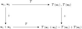
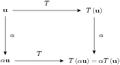
Here are two diagrams that convey the essence of the two defining properties of a linear transformation. In each case, begin in the upper left-hand corner, and follow the arrows around the rectangle to the lower-right hand corner, taking two different routes and doing the indicated operations labeled on the arrows. There are two results there. For a linear transformation these two expressions are always equal.
A couple of words about notation. T is the name of the linear transformation, and should be used when we want to discuss the function as a whole. T\left (u\right ) is how we talk about the output of the function, it is a vector in the vector space V . When we write T\left (x + y\right ) = T\left (x\right ) + T\left (y\right ), the plus sign on the left is the operation of vector addition in the vector space U, since x and y are elements of U. The plus sign on the right is the operation of vector addition in the vector space V , since T\left (x\right ) and T\left (y\right ) are elements of the vector space V . These two instances of vector addition might be wildly different.
Let’s examine several examples and begin to form a catalog of known linear transformations to work with.
Example ALT
A linear transformation
Define T : {ℂ}^{3}\mathrel{↦}{ℂ}^{2}
by describing the output of the function for a generic input with the formula
|
T\left (\left [\array{
{x}_{1}
\cr
{x}_{2}
\cr
{x}_{3} } \right ]\right ) = \left [\array{
2{x}_{1} + {x}_{3}
\cr
−4{x}_{2} } \right ]
|
and check the two defining properties.
So by Definition LT, T is a linear transformation. ⊠
It can be just as instructive to look at functions that are not linear transformations. Since the defining conditions must be true for all vectors and scalars, it is enough to find just one situation where the properties fail.
Example NLT
Not a linear transformation
Define S : {ℂ}^{3}\mathrel{↦}{ℂ}^{3}
by
|
S\left (\left [\array{
{x}_{1}
\cr
{x}_{2}
\cr
{x}_{3} } \right ]\right ) = \left [\array{
4{x}_{1} + 2{x}_{2}
\cr
0
\cr
{x}_{1} + 3{x}_{3} − 2 } \right ]
|
This function “looks” linear, but consider
So the second required property fails for the choice of α = 3 and x = \left [\array{ 1 \cr 2 \cr 3 } \right ]and by Definition LT, S is not a linear transformation. It is just about as easy to find an example where the first defining property fails (try it!). Notice that it is the “-2” in the third component of the definition of S that prevents the function from being a linear transformation. ⊠
Example LTPM
Linear transformation, polynomials to matrices
Define a linear transformation T : {P}_{3}\mathrel{↦}{M}_{22}
by
|
T\left (a + bx + c{x}^{2} + d{x}^{3}\right ) = \left [\array{
a + b&a − 2c
\cr
d & b − d } \right ]
|
We verify the two defining conditions of a linear transformations.
So by Definition LT, T is a linear transformation. ⊠
Example LTPP
Linear transformation, polynomials to polynomials
Define a function S : {P}_{4}\mathrel{↦}{P}_{5}
by
|
S(p(x)) = (x − 2)p(x)
|
Then
So by Definition LT, S is a linear transformation. ⊠
Linear transformations have many amazing properties, which we will investigate through the next few sections. However, as a taste of things to come, here is a theorem we can prove now and put to use immediately.
Theorem LTTZZ
Linear Transformations Take Zero to Zero
Suppose T : U\mathrel{↦}V is a linear
transformation. Then T\left (0\right ) = 0.
□
Proof The two zero vectors in the conclusion of the theorem are different. The first is from U while the second is from V . We will subscript the zero vectors in this proof to highlight the distinction. Think about your objects. (This proof is contributed by Mark Shoemaker).
Return to Example NLT and compute S\left (\left [\array{ 0 \cr 0 \cr 0 } \right ]\right ) = \left [\array{ 0 \cr 0 \cr −2 } \right ] to quickly see again that S is not a linear transformation, while in Example LTPM compute S\left (0 + 0x + 0{x}^{2} + 0{x}^{3}\right ) = \left [\array{ 0&0 \cr 0&0 } \right ]as an example of Theorem LTTZZ at work.
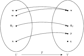
Throughout this chapter, and Chapter R, we will include drawings of linear transformations. We will call them “cartoons,” not because they are humorous, but because they will only expose a portion of the truth. A Bugs Bunny cartoon might give us some insights on human nature, but the rules of physics and biology are routinely (and grossly) violated. So it will be with our linear transformation cartoons. Here is our first, followed by a guide to help you understand how these are meant to describe fundamental truths about linear transformations, while simultaneously violating other truths.
Here we picture a linear transformation T : U\mathrel{↦}V , where this information will be consistently displayed along the bottom edge. The ovals are meant to represent the vector spaces, in this case U, the domain, on the left and V , the codomain, on the right. Of course, vector spaces are typically infinite sets, so you’ll have to imagine that characteristic of these sets. A small dot inside of an oval will represent a vector within that vector space, sometimes with a name, sometimes not (in this case every vector has a name). The sizes of the ovals are meant to be proportional to the dimensions of the vector spaces. However, when we make no assumptions about the dimensions, we will draw the ovals as the same size, as we have done here (which is not meant to suggest that the dimensions have to be equal).
To convey that the linear transformation associates a certain input with a certain output, we will draw an arrow from the input to the output. So, for example, in this cartoon we suggest that T\left (x\right ) = y. Nothing in the definition of a linear transformation prevents two different inputs being sent to the same output and we see this in T\left (u\right ) = v = T\left (w\right ). Similarly, an output may not have any input being sent its way, as illustrated by no arrow pointing at t. In this cartoon, we have captured the essence of our one general theorem about linear transformations, Theorem LTTZZ, T\left ({0}_{U}\right ) = {0}_{V }. On occasion we might include this basic fact when it is relevant, at other times maybe not. Note that the definition of a linear transformation requires that it be a function, so every element of the domain should be associated with some element of the codomain. This will be reflected by never having an element of the domain without an arrow originating there.
These cartoons are of course no substitute for careful definitions and proofs, but they can be a handy way to think about the various properties we will be studying.
If you give me a matrix, then I can quickly build you a linear transformation. Always. First a motivating example and then the theorem.
Example LTM
Linear transformation from a matrix
Let
|
A = \left [\array{
3&−1&8& 1
\cr
2& 0 &5&−2
\cr
1& 1 &3&−7 } \right ]
|
and define a function P : {ℂ}^{4}\mathrel{↦}{ℂ}^{3} by
|
P\left (x\right ) = Ax
|
So we are using an old friend, the matrix-vector product (Definition MVP) as a way to convert a vector with 4 components into a vector with 3 components. Applying Definition MVP allows us to write the defining formula for P in a slightly different form,
|
P\left (x\right ) = Ax = \left [\array{
3&−1&8& 1
\cr
2& 0 &5&−2
\cr
1& 1 &3&−7 } \right ]\left [\array{
{x}_{1}
\cr
{x}_{2}
\cr
{x}_{3}
\cr
{x}_{4} } \right ] = {x}_{1}\left [\array{
3
\cr
2
\cr
1 } \right ]+{x}_{2}\left [\array{
−1
\cr
0
\cr
1 } \right ]+{x}_{3}\left [\array{
8
\cr
5
\cr
3 } \right ]+{x}_{4}\left [\array{
1
\cr
−2
\cr
−7 } \right ]
|
So we recognize the action of the function P as using the components of the vector ({x}_{1},\kern 1.95872pt {x}_{2},\kern 1.95872pt {x}_{3},\kern 1.95872pt {x}_{4}) as scalars to form the output of P as a linear combination of the four columns of the matrix A, which are all members of {ℂ}^{3}, so the result is a vector in {ℂ}^{3}. We can rearrange this expression further, using our definitions of operations in {ℂ}^{3} (Section VO).
You might recognize this final expression as being similar in style to some previous examples (Example ALT) and some linear transformations defined in the archetypes (Archetype M through Archetype R). But the expression that says the output of this linear transformation is a linear combination of the columns of A is probably the most powerful way of thinking about examples of this type.
Almost forgot — we should verify that P is indeed a linear transformation. This is easy with two matrix properties from Section MM.
}
So by Definition LT, P is a linear transformation. ⊠
So the multiplication of a vector by a matrix “transforms” the input vector into an output vector, possibly of a different size, by performing a linear combination. And this transformation happens in a “linear” fashion. This “functional” view of the matrix-vector product is the most important shift you can make right now in how you think about linear algebra. Here’s the theorem, whose proof is very nearly an exact copy of the verification in the last example.
Theorem MBLT
Matrices Build Linear Transformations
Suppose that A
is an m × n matrix.
Define a function T : {ℂ}^{n}\mathrel{↦}{ℂ}^{m}
by T\left (x\right ) = Ax. Then
T is a linear
transformation. □
Proof
}
So by Definition LT, T is a linear transformation. ■
So Theorem MBLT gives us a rapid way to construct linear transformations. Grab an m × n matrix A, define T\left (x\right ) = Ax and Theorem MBLT tells us that T is a linear transformation from {ℂ}^{n} to {ℂ}^{m}, without any further checking.
We can turn Theorem MBLT around. You give me a linear transformation and I will give you a matrix.
Example MFLT
Matrix from a linear transformation
Define the function R: {ℂ}^{3}\mathrel{↦}{ℂ}^{4}
by
|
R\left (\left [\array{
{x}_{1}
\cr
{x}_{2}
\cr
{x}_{3} } \right ]\right ) = \left [\array{
2{x}_{1} − 3{x}_{2} + 4{x}_{3}
\cr
{x}_{1} + {x}_{2} + {x}_{3}
\cr
−{x}_{1} + 5{x}_{2} − 3{x}_{3}
\cr
{x}_{2} − 4{x}_{3} } \right ]
|
You could verify that R is a linear transformation by applying the definition, but we will instead massage the expression defining a typical output until we recognize the form of a known class of linear transformations.
So if we define the matrix
|
B = \left [\array{
2 &−3& 4
\cr
1 & 1 & 1
\cr
−1& 5 &−3
\cr
0 & 1 &−4 } \right ]
|
then R\left (x\right ) = Bx. By Theorem MBLT, we can easily recognize R as a linear transformation since it has the form described in the hypothesis of the theorem. ⊠
Example MFLT was not accident. Consider any one of the archetypes where both the domain and codomain are sets of column vectors (Archetype M through Archetype R) and you should be able to mimic the previous example. Here’s the theorem, which is notable since it is our first occasion to use the full power of the defining properties of a linear transformation when our hypothesis includes a linear transformation.
Theorem MLTCV
Matrix of a Linear Transformation, Column Vectors
Suppose that T : {ℂ}^{n}\mathrel{↦}{ℂ}^{m}
is a linear transformation. Then there is an
m × n matrix
A such
that T\left (x\right ) = Ax.
□
Proof The conclusion says a certain matrix exists. What better way to prove something exists than to actually build it? So our proof will be constructive (Technique C), and the procedure that we will use abstractly in the proof can be used concretely in specific examples.
Let {e}_{1},\kern 1.95872pt {e}_{2},\kern 1.95872pt {e}_{3},\kern 1.95872pt \mathop{\mathop{…}},\kern 1.95872pt {e}_{n} be the columns of the identity matrix of size n, {I}_{n} (Definition SUV). Evaluate the linear transformation T with each of these standard unit vectors as an input, and record the result. In other words, define n vectors in {ℂ}^{m}, {A}_{i}, 1 ≤ i ≤ n by
|
{A}_{i} = T\left ({e}_{i}\right )
|
Then package up these vectors as the columns of a matrix
|
A = \left [{A}_{1}|{A}_{2}|{A}_{3}|\mathop{\mathop{…}}|{A}_{n}\right ]
|
Does A have the desired properties? First, A is clearly an m × n matrix. Then
as desired. ■
So if we were to restrict our study of linear transformations to those where the domain and codomain are both vector spaces of column vectors (Definition VSCV), every matrix leads to a linear transformation of this type (Theorem MBLT), while every such linear transformation leads to a matrix (Theorem MLTCV). So matrices and linear transformations are fundamentally the same. We call the matrix A of Theorem MLTCV the matrix representation of T.
We have defined linear transformations for more general vector spaces than just {ℂ}^{m}, can we extend this correspondence between linear transformations and matrices to more general linear transformations (more general domains and codomains)? Yes, and this is the main theme of Chapter R. Stay tuned. For now, let’s illustrate Theorem MLTCV with an example.
Example MOLT
Matrix of a linear transformation
Suppose S : {ℂ}^{3}\mathrel{↦}{ℂ}^{4}
is defined by
|
S\left (\left [\array{
{x}_{1}
\cr
{x}_{2}
\cr
{x}_{3} } \right ]\right ) = \left [\array{
3{x}_{1} − 2{x}_{2} + 5{x}_{3}
\cr
{x}_{1} + {x}_{2} + {x}_{3}
\cr
9{x}_{1} − 2{x}_{2} + 5{x}_{3}
\cr
4{x}_{2} } \right ]
|
Then
so define
|
C = \left [{C}_{1}|{C}_{2}|{C}_{3}\right ] = \left [\array{
3&−2&5
\cr
1& 1 &1
\cr
9&−2&5
\cr
0& 4 &0 } \right ]
|
and Theorem MLTCV guarantees that S\left (x\right ) = Cx.
As an illuminating exercise, let z = \left [\array{ 2 \cr −3 \cr 3 } \right ] and compute S\left (z\right ) two different ways. First, return to the definition of S and evaluate S\left (z\right ) directly. Then do the matrix-vector product Cz. In both cases you should obtain the vector S\left (z\right ) = \left [\array{ 27 \cr 2 \cr 39 \cr −12 } \right ]. ⊠
It is the interaction between linear transformations and linear combinations that lies at the heart of many of the important theorems of linear algebra. The next theorem distills the essence of this. The proof is not deep, the result is hardly startling, but it will be referenced frequently. We have already passed by one occasion to employ it, in the proof of Theorem MLTCV. Paraphrasing, this theorem says that we can “push” linear transformations “down into” linear combinations, or “pull” linear transformations “up out” of linear combinations. We’ll have opportunities to both push and pull.
Theorem LTLC
Linear Transformations and Linear Combinations
Suppose that T : U\mathrel{↦}V is a
linear transformation, {u}_{1},\kern 1.95872pt {u}_{2},\kern 1.95872pt {u}_{3},\kern 1.95872pt \mathop{\mathop{…}},\kern 1.95872pt {u}_{t}
are vectors from U
and {a}_{1},\kern 1.95872pt {a}_{2},\kern 1.95872pt {a}_{3},\kern 1.95872pt \mathop{\mathop{…}},\kern 1.95872pt {a}_{t} are
scalars from {ℂ}^{}.
Then
|
T\left ({a}_{1}{u}_{1} + {a}_{2}{u}_{2} + {a}_{3}{u}_{3} + \mathrel{⋯} + {a}_{t}{u}_{t}\right ) = {a}_{1}T\left ({u}_{1}\right )+{a}_{2}T\left ({u}_{2}\right )+{a}_{3}T\left ({u}_{3}\right )+\mathrel{⋯}+{a}_{t}T\left ({u}_{t}\right )
|
Proof
Some authors, especially in more advanced texts, take the conclusion of Theorem LTLC as the defining condition of a linear transformation. This has the appeal of being a single condition, rather than the two-part condition of Definition LT. (See Exercise LT.T20).
Our next theorem says, informally, that it is enough to know how a linear transformation behaves for inputs from any basis of the domain, and all the other outputs are described by a linear combination of these few values. Again, the statement of the theorem, and its proof, are not remarkable, but the insight that goes along with it is very fundamental.
Theorem LTDB
Linear Transformation Defined on a Basis
Suppose B = \left \{{u}_{1},\kern 1.95872pt {u}_{2},\kern 1.95872pt {u}_{3},\kern 1.95872pt \mathop{\mathop{…}},\kern 1.95872pt {u}_{n}\right \} is a basis
for the vector space U
and {v}_{1},\kern 1.95872pt {v}_{2},\kern 1.95872pt {v}_{3},\kern 1.95872pt \mathop{\mathop{…}},\kern 1.95872pt {v}_{n} is a list of vectors
from the vector space V
(which are not necessarily distinct). Then there is a unique linear transformation,
T : U\mathrel{↦}V , such
that T\left ({u}_{i}\right ) = {v}_{i},
1 ≤ i ≤ n.
□
Proof To prove the existence of T, we construct a function and show that it is a linear transformation (Technique C). Suppose w ∈ U is an arbitrary element of the domain. Then by Theorem VRRB there are unique scalars {a}_{1},\kern 1.95872pt {a}_{2},\kern 1.95872pt {a}_{3},\kern 1.95872pt \mathop{\mathop{…}},\kern 1.95872pt {a}_{n} such that
}
It should be clear that T behaves as required for n inputs from B. Since the scalars provided by Theorem VRRB are unique, there is no ambiguity in this definition, and T qualifies as a function with domain U and codomain V (i.e. T is well-defined). But is T a linear transformation as well?
Let x ∈ U be a second element of the domain, and suppose the scalars provided by Theorem VRRB (relative to B) are {b}_{1},\kern 1.95872pt {b}_{2},\kern 1.95872pt {b}_{3},\kern 1.95872pt \mathop{\mathop{…}},\kern 1.95872pt {b}_{n}. Then
Let α ∈ ℂ be any scalar. Then
So by Definition LT, T is a linear transformation.
Is T unique (among all linear transformations that take the {u}_{i} to the {v}_{i})? Applying Technique U, we posit the existence of a second linear transformation, S : U\mathrel{↦}V such that S\left ({u}_{i}\right ) = {v}_{i}, 1 ≤ i ≤ n. Again, let w ∈ U represent an arbitrary element of U and let {a}_{1},\kern 1.95872pt {a}_{2},\kern 1.95872pt {a}_{3},\kern 1.95872pt \mathop{\mathop{…}},\kern 1.95872pt {a}_{n} be the scalars provided by Theorem VRRB (relative to B). We have,
So the output of T and S agree on every input, which means they are equal as functions, T = S. So T is unique. ■
You might recall facts from analytic geometry, such as “any two points determine a line” and “any three non-collinear points determine a parabola.” Theorem LTDB has much of the same feel. By specifying the n outputs for inputs from a basis, an entire linear transformation is determined. The analogy is not perfect, but the style of these facts are not very dissimilar from Theorem LTDB.
Notice that the statement of Theorem LTDB asserts the existence of a linear transformation with certain properties, while the proof shows us exactly how to define the desired linear transformation. The next examples how how to work with linear transformations that we find this way.
Example LTDB1
Linear transformation defined on a basis
Consider the linear transformation T : {ℂ}^{3}\mathrel{↦}{ℂ}^{2}
that is required to have the following three values,
Because
|
B = \left \{\left [\array{
1
\cr
0
\cr
0 } \right ],\kern 1.95872pt \left [\array{
0
\cr
1
\cr
0 } \right ],\kern 1.95872pt \left [\array{
0
\cr
0
\cr
1 } \right ]\right \}
|
is a basis for {ℂ}^{3} (Theorem SUVB), Theorem LTDB says there is a unique linear transformation T that behaves this way. How do we compute other values of T? Consider the input
|
w = \left [\array{
2
\cr
−3
\cr
1 } \right ] = (2)\left [\array{
1
\cr
0
\cr
0 } \right ]+(−3)\left [\array{
0
\cr
1
\cr
0 } \right ]+(1)\left [\array{
0
\cr
0
\cr
1 } \right ]
|
Then
|
T\left (w\right ) = (2)\left [\array{
2
\cr
1 } \right ]+(−3)\left [\array{
−1
\cr
4 } \right ]+(1)\left [\array{
6
\cr
0 } \right ] = \left [\array{
13
\cr
−10 } \right ]
|
Doing it again,
|
x = \left [\array{
5
\cr
2
\cr
−3 } \right ] = (5)\left [\array{
1
\cr
0
\cr
0 } \right ]+(2)\left [\array{
0
\cr
1
\cr
0 } \right ]+(−3)\left [\array{
0
\cr
0
\cr
1 } \right ]
|
so
|
T\left (x\right ) = (5)\left [\array{
2
\cr
1 } \right ]+(2)\left [\array{
−1
\cr
4 } \right ]+(−3)\left [\array{
6
\cr
0 } \right ] = \left [\array{
−10
\cr
13} \right ]
|
Any other value of T could be computed in a similar manner. So rather than being given a formula for the outputs of T, the requirement that T behave in a certain way for the inputs chosen from a basis of the domain, is as sufficient as a formula for computing any value of the function. You might notice some parallels between this example and Example MOLT or Theorem MLTCV. ⊠
Example LTDB2
Linear transformation defined on a basis
Consider the linear transformation R: {ℂ}^{3}\mathrel{↦}{ℂ}^{2}
with the three values,
You can check that
|
D = \left \{\left [\array{
1
\cr
2
\cr
1 } \right ],\kern 1.95872pt \left [\array{
−1
\cr
5
\cr
1 } \right ],\kern 1.95872pt \left [\array{
3
\cr
1
\cr
4 } \right ]\right \}
|
is a basis for {ℂ}^{3} (make the vectors the columns of a square matrix and check that the matrix is nonsingular, Theorem CNMB). By Theorem LTDB we know there is a unique linear transformation R with the three specified outputs. However, we have to work just a bit harder to take an input vector and express it as a linear combination of the vectors in D. For example, consider,
|
y = \left [\array{
8
\cr
−3
\cr
5 } \right ]
|
Then we must first write y as a linear combination of the vectors in D and solve for the unknown scalars, to arrive at
|
y = \left [\array{
8
\cr
−3
\cr
5 } \right ] = (3)\left [\array{
1
\cr
2
\cr
1 } \right ]+(−2)\left [\array{
−1
\cr
5
\cr
1 } \right ]+(1)\left [\array{
3
\cr
1
\cr
4 } \right ]
|
Then the proof of Theorem LTDB gives us
|
R\left (y\right ) = (3)\left [\array{
5
\cr
−1 } \right ]+(−2)\left [\array{
0
\cr
4 } \right ]+(1)\left [\array{
2
\cr
3 } \right ] = \left [\array{
17
\cr
−8 } \right ]
|
Any other value of R could be computed in a similar manner. ⊠
Here is a third example of a linear transformation defined by its action on a basis, only with more abstract vector spaces involved.
Example LTDB3
Linear transformation defined on a basis
The set W = \left \{p(x) ∈ {P}_{3}\mathrel{∣}p(1) = 0,p(3) = 0\right \} ⊆ {P}_{3}
is a subspace of the vector space of polynomials
{P}_{3}. This
subspace has C = \left \{3 − 4x + {x}^{2},\kern 1.95872pt 12 − 13x + {x}^{3}\right \}
as a basis (check this!). Suppose we consider the linear transformation
S : {P}_{3}\mathrel{↦}{M}_{22} with
values
By Theorem LTDB we know there is a unique linear transformation with these two values. To illustrate a sample computation of S, consider q(x) = 9 − 6x − 5{x}^{2} + 2{x}^{3}. Verify that q(x) is an element of W (does it have roots at x = 1 and x = 3?), then find the scalars needed to write it as a linear combination of the basis vectors in C. Because
|
q(x) = 9 − 6x − 5{x}^{2} + 2{x}^{3} = (−5)(3 − 4x + {x}^{2}) + (2)(12 − 13x + {x}^{3})
|
The proof of Theorem LTDB gives us
|
S\left (q\right ) = (−5)\left [\array{
1&−3
\cr
2& 0} \right ]+(2)\left [\array{
0&1
\cr
1&0 } \right ] = \left [\array{
−5&17
\cr
−8& 0 } \right ]
|
And all the other outputs of S could be computed in the same manner. Every output of S will have a zero in the second row, second column. Can you see why this is so? ⊠
Informally, we can describe Theorem LTDB by saying “it is enough to know what a linear transformation does to a basis (of the domain).”
The definition of a function requires that for each input in the domain there is exactly one output in the codomain. However, the correspondence does not have to behave the other way around. A member of the codomain might have many inputs from the domain that create it, or it may have none at all. To formalize our discussion of this aspect of linear transformations, we define the pre-image.
Definition PI
Pre-Image
Suppose that T : U\mathrel{↦}V is a linear
transformation. For each v,
define the pre-image of v
to be the subset of U
given by
|
{T}^{−1}\left (v\right ) = \left \{u ∈ U\mathrel{∣}T\left (u\right ) = v\right \}
|
In other words, {T}^{−1}\left (v\right ) is the set of all those vectors in the domain U that get “sent” to the vector v.
Example SPIAS
Sample pre-images, Archetype S
Archetype S is the linear transformation defined by
|
T : {ℂ}^{3}\mathrel{↦}{M}_{
22},\quad T\left (\left [\array{
a
\cr
b
\cr
c } \right ]\right ) = \left [\array{
a − b & 2a + 2b + c
\cr
3a + b + c&−2a − 6b − 2c } \right ]
|
We could compute a pre-image for every element of the codomain {M}_{22}. However, even in a free textbook, we do not have the room to do that, so we will compute just two.
Choose
|
v = \left [\array{
2&1
\cr
3&2 } \right ] ∈ {M}_{22}
|
for no particular reason. What is {T}^{−1}\left (v\right )? Suppose u = \left [\array{ {u}_{1} \cr {u}_{2} \cr {u}_{3} } \right ] ∈ {T}^{−1}\left (v\right ). The condition that T\left (u\right ) = v becomes
|
\left [\array{
2&1
\cr
3&2 } \right ] = v = T\left (u\right ) = T\left (\left [\array{
{u}_{1}
\cr
{u}_{2}
\cr
{u}_{3} } \right ]\right ) = \left [\array{
{u}_{1} − {u}_{2} & 2{u}_{1} + 2{u}_{2} + {u}_{3}
\cr
3{u}_{1} + {u}_{2} + {u}_{3}&−2{u}_{1} − 6{u}_{2} − 2{u}_{3} } \right ]
|
Using matrix equality (Definition ME), we arrive at a system of four equations in the three unknowns {u}_{1},\kern 1.95872pt {u}_{2},\kern 1.95872pt {u}_{3} with an augmented matrix that we can row-reduce in the hunt for solutions,
|
\left [\array{
1 &−1& 0 &2
\cr
2 & 2 & 1 &1
\cr
3 & 1 & 1 &3
\cr
−2&−6&−2&2 } \right ]\mathop{\longrightarrow}\limits_{}^{\text{RREF}}\left [\array{
\text{1}&0&{1\over
4}& {5\over
4}
\cr
0&\text{1}&{1\over
4}&−{3\over
4}
\cr
0&0&0& 0
\cr
0&0&0& 0 } \right ]
|
We recognize this system as having infinitely many solutions described by the single free variable {u}_{3}. Eventually obtaining the vector form of the solutions (Theorem VFSLS), we can describe the preimage precisely as,
This last line is merely a suggestive way of describing the set on the previous line. You might create three or four vectors in the preimage, and evaluate T with each. Was the result what you expected? For a hint of things to come, you might try evaluating T with just the lone vector in the spanning set above. What was the result? Now take a look back at Theorem PSPHS. Hmmmm.
OK, let’s compute another preimage, but with a different outcome this time. Choose
|
v = \left [\array{
1&1
\cr
2&4 } \right ] ∈ {M}_{22}
|
What is {T}^{−1}\left (v\right )? Suppose u = \left [\array{ {u}_{1} \cr {u}_{2} \cr {u}_{3} } \right ] ∈ {T}^{−1}\left (v\right ). That T\left (u\right ) = v becomes
|
\left [\array{
1&1
\cr
2&4 } \right ] = v = T\left (u\right ) = T\left (\left [\array{
{u}_{1}
\cr
{u}_{2}
\cr
{u}_{3} } \right ]\right ) = \left [\array{
{u}_{1} − {u}_{2} & 2{u}_{1} + 2{u}_{2} + {u}_{3}
\cr
3{u}_{1} + {u}_{2} + {u}_{3}&−2{u}_{1} − 6{u}_{2} − 2{u}_{3} } \right ]
|
Using matrix equality (Definition ME), we arrive at a system of four equations in the three unknowns {u}_{1},\kern 1.95872pt {u}_{2},\kern 1.95872pt {u}_{3} with an augmented matrix that we can row-reduce in the hunt for solutions,
|
\left [\array{
1 &−1& 0 &1
\cr
2 & 2 & 1 &1
\cr
3 & 1 & 1 &2
\cr
−2&−6&−2&4 } \right ]\mathop{\longrightarrow}\limits_{}^{\text{RREF}}\left [\array{
\text{1}&0&{1\over
4}&0
\cr
0&\text{1}&{1\over
4}&0
\cr
0&0&0&\text{1}
\cr
0&0&0&0 } \right ]
|
By Theorem RCLS we recognize this system as inconsistent. So no vector u is a member of {T}^{−1}\left (v\right ) and so
|
{T}^{−1}\left (v\right ) = ∅
|
The preimage is just a set, it is almost never a subspace of U (you might think about just when {T}^{−1}\left (v\right ) is a subspace, see Exercise ILT.T10). We will describe its properties going forward, and it will be central to the main ideas of this chapter.
We can combine linear transformations in natural ways to create new linear transformations. So we will define these combinations and then prove that the results really are still linear transformations. First the sum of two linear transformations.
Definition LTA
Linear Transformation Addition
Suppose that T : U\mathrel{↦}V
and S : U\mathrel{↦}V are
two linear transformations with the same domain and codomain. Then their sum is the
function T + S : U\mathrel{↦}V
whose outputs are defined by
|
(T + S)\left (u\right ) = T\left (u\right ) + S\left (u\right )
|
Notice that the first plus sign in the definition is the operation being defined, while the second one is the vector addition in V . (Vector addition in U will appear just now in the proof that T + S is a linear transformation.) Definition LTA only provides a function. It would be nice to know that when the constituents (T, S) are linear transformations, then so too is T + S.
Theorem SLTLT
Sum of Linear Transformations is a Linear Transformation
Suppose that T : U\mathrel{↦}V
and S : U\mathrel{↦}V
are two linear transformations with the same domain and codomain. Then
T + S : U\mathrel{↦}V is a linear
transformation. □
Proof We simply check the defining properties of a linear transformation (Definition LT). This is a good place to consistently ask yourself which objects are being combined with which operations.
Example STLT
Sum of two linear transformations
Suppose that T : {ℂ}^{2}\mathrel{↦}{ℂ}^{3}
and S : {ℂ}^{2}\mathrel{↦}{ℂ}^{3}
are defined by
Then by Definition LTA, we have
|
(T+S)\left (\left [\array{
{x}_{1}
\cr
{x}_{2} } \right ]\right ) = T\left (\left [\array{
{x}_{1}
\cr
{x}_{2} } \right ]\right )+S\left (\left [\array{
{x}_{1}
\cr
{x}_{2} } \right ]\right ) = \left [\array{
{x}_{1} + 2{x}_{2}
\cr
3{x}_{1} − 4{x}_{2}
\cr
5{x}_{1} + 2{x}_{2} } \right ]+\left [\array{
4{x}_{1} − {x}_{2}
\cr
{x}_{1} + 3{x}_{2}
\cr
−7{x}_{1} + 5{x}_{2} } \right ] = \left [\array{
5{x}_{1} + {x}_{2}
\cr
4{x}_{1} − {x}_{2}
\cr
−2{x}_{1} + 7{x}_{2} } \right ]
|
and by Theorem SLTLT we know T + S is also a linear transformation from {ℂ}^{2} to {ℂ}^{3}. ⊠
Definition LTSM
Linear Transformation Scalar Multiplication
Suppose that T : U\mathrel{↦}V is a linear
transformation and α ∈ {ℂ}^{}.
Then the scalar multiple is the function
αT : U\mathrel{↦}V
whose outputs are defined by
|
(αT)\left (u\right ) = αT\left (u\right )
|
Given that T is a linear transformation, it would be nice to know that αT is also a linear transformation.
Theorem MLTLT
Multiple of a Linear Transformation is a Linear Transformation
Suppose that T : U\mathrel{↦}V is a linear
transformation and α ∈ {ℂ}^{}.
Then (αT): U\mathrel{↦}V is a linear
transformation. □
Proof We simply check the defining properties of a linear transformation (Definition LT). This is another good place to consistently ask yourself which objects are being combined with which operations.
Example SMLT
Scalar multiple of a linear transformation
Suppose that T : {ℂ}^{4}\mathrel{↦}{ℂ}^{3}
is defined by
|
T\left (\left [\array{
{x}_{1}
\cr
{x}_{2}
\cr
{x}_{3}
\cr
{x}_{4} } \right ]\right ) = \left [\array{
{x}_{1} + 2{x}_{2} − {x}_{3} + 2{x}_{4}
\cr
{x}_{1} + 5{x}_{2} − 3{x}_{3} + {x}_{4}
\cr
−2{x}_{1} + 3{x}_{2} − 4{x}_{3} + 2{x}_{4} } \right ]
|
For the sake of an example, choose α = 2, so by Definition LTSM, we have
|
αT\left (\left [\array{
{x}_{1}
\cr
{x}_{2}
\cr
{x}_{3}
\cr
{x}_{4} } \right ]\right ) = 2T\left (\left [\array{
{x}_{1}
\cr
{x}_{2}
\cr
{x}_{3}
\cr
{x}_{4} } \right ]\right ) = 2\left [\array{
{x}_{1} + 2{x}_{2} − {x}_{3} + 2{x}_{4}
\cr
{x}_{1} + 5{x}_{2} − 3{x}_{3} + {x}_{4}
\cr
−2{x}_{1} + 3{x}_{2} − 4{x}_{3} + 2{x}_{4} } \right ] = \left [\array{
2{x}_{1} + 4{x}_{2} − 2{x}_{3} + 4{x}_{4}
\cr
2{x}_{1} + 10{x}_{2} − 6{x}_{3} + 2{x}_{4}
\cr
−4{x}_{1} + 6{x}_{2} − 8{x}_{3} + 4{x}_{4} } \right ]
|
and by Theorem MLTLT we know 2T is also a linear transformation from {ℂ}^{4} to {ℂ}^{3}. ⊠
Now, let’s imagine we have two vector spaces, U and V , and we collect every possible linear transformation from U to V into one big set, and call it ℒT\left (U,\kern 1.95872pt V \right ). Definition LTA and Definition LTSM tell us how we can “add” and “scalar multiply” two elements of ℒT\left (U,\kern 1.95872pt V \right ). Theorem SLTLT and Theorem MLTLT tell us that if we do these operations, then the resulting functions are linear transformations that are also in ℒT\left (U,\kern 1.95872pt V \right ). Hmmmm, sounds like a vector space to me! A set of objects, an addition and a scalar multiplication. Why not?
Theorem VSLT
Vector Space of Linear Transformations
Suppose that U
and V
are vector spaces. Then the set of all linear transformations from
U to
V ,
ℒT\left (U,\kern 1.95872pt V \right ) is a vector
space when the operations are those given in Definition LTA and Definition LTSM.
□
Proof Theorem SLTLT and Theorem MLTLT provide two of the ten properties in Definition VS. However, we still need to verify the remaining eight properties. By and large, the proofs are straightforward and rely on concocting the obvious object, or by reducing the question to the same vector space property in the vector space V .
The zero vector is of some interest, though. What linear transformation would we add to any other linear transformation, so as to keep the second one unchanged? The answer is Z : U\mathrel{↦}V defined by Z\left (u\right ) = {0}_{V } for every u ∈ U. Notice how we do not need to know any of the specifics about U and V to make this definition of Z. ■
Definition LTC
Linear Transformation Composition
Suppose that T : U\mathrel{↦}V
and S : V \mathrel{↦}W
are linear transformations. Then the composition of
S and
T is the
function (S ∘ T): U\mathrel{↦}W
whose outputs are defined by
|
(S ∘ T)\left (u\right ) = S\left (T\left (u\right )\right )
|
Given that T and S are linear transformations, it would be nice to know that S ∘ T is also a linear transformation.
Theorem CLTLT
Composition of Linear Transformations is a Linear Transformation
Suppose that T : U\mathrel{↦}V
and S : V \mathrel{↦}W are linear
transformations. Then (S ∘ T): U\mathrel{↦}W is
a linear transformation. □
Proof We simply check the defining properties of a linear transformation (Definition LT).
}
Example CTLT
Composition of two linear transformations
Suppose that T : {ℂ}^{2}\mathrel{↦}{ℂ}^{4}
and S : {ℂ}^{4}\mathrel{↦}{ℂ}^{3}
are defined by
Then by Definition LTC
and by Theorem CLTLT S ∘ T is a linear transformation from {ℂ}^{2} to {ℂ}^{3}. ⊠
Here is an interesting exercise that will presage an important result later. In Example STLT compute (via Theorem MLTCV) the matrix of T, S and T + S. Do you see a relationship between these three matrices?
In Example SMLT compute (via Theorem MLTCV) the matrix of T and 2T. Do you see a relationship between these two matrices?
Here’s the tough one. In Example CTLT compute (via Theorem MLTCV) the matrix of T, S and S ∘ T. Do you see a relationship between these three matrices???
|
T : {ℂ}^{3}\mathrel{↦}{ℂ}^{2},\quad T\left (\left [\array{
{x}_{1}
\cr
{x}_{2}
\cr
{x}_{3}
} \right ]\right ) = \left [\array{
3{x}_{1} − {x}_{2} + {x}_{3}
\cr
8{x}_{2} − 6
} \right ]
|
|
S : {ℂ}^{2}\mathrel{↦}{ℂ}^{3},\quad S\left (\left [\array{
{x}_{1}
\cr
{x}_{2}
} \right ]\right ) = \left [\array{
3{x}_{1} + 5{x}_{2}
\cr
8{x}_{1} − 3{x}_{2}
\cr
−4{x}_{1}
} \right ]
|
C15 The archetypes below are all linear transformations whose domains and
codomains are vector spaces of column vectors (Definition VSCV). For
each one, compute the matrix representation described in the proof of
Theorem MLTCV.
Archetype M
Archetype N
Archetype O
Archetype P
Archetype Q
Archetype R
Contributed by Robert Beezer
C20 Let w = \left [\array{
−3
\cr
1
\cr
4 } \right ]. Referring to
Example MOLT, compute S\left (w\right )
two different ways. First use the definition of
S, then compute the
matrix-vector product Cw
(Definition MVP).
Contributed by Robert Beezer Solution [1375]
C25 Define the linear transformation
|
T : {ℂ}^{3}\mathrel{↦}{ℂ}^{2},\quad T\left (\left [\array{
{x}_{1}
\cr
{x}_{2}
\cr
{x}_{3} } \right ]\right ) = \left [\array{
2{x}_{1} − {x}_{2} + 5{x}_{3}
\cr
−4{x}_{1} + 2{x}_{2} − 10{x}_{3} } \right ]
|
Verify that T
is a linear transformation.
Contributed by Robert Beezer Solution [1375]
C26 Verify that the function below is a linear transformation.
|
T : {P}_{2}\mathrel{↦}{ℂ}^{2},\quad T\left (a + bx + c{x}^{2}\right ) = \left [\array{
2a − b
\cr
b + c } \right ]
|
Contributed by Robert Beezer Solution [1375]
C30 Define the linear transformation
|
T : {ℂ}^{3}\mathrel{↦}{ℂ}^{2},\quad T\left (\left [\array{
{x}_{1}
\cr
{x}_{2}
\cr
{x}_{3} } \right ]\right ) = \left [\array{
2{x}_{1} − {x}_{2} + 5{x}_{3}
\cr
−4{x}_{1} + 2{x}_{2} − 10{x}_{3} } \right ]
|
Compute the preimages, {T}^{−1}\left (\left [\array{
2
\cr
3 } \right ]\right )
and {T}^{−1}\left (\left [\array{
4
\cr
−8 } \right ]\right ).
Contributed by Robert Beezer Solution [1376]
C31 For the linear transformation S compute the pre-images.
M10 Define two linear transformations, T : {ℂ}^{4}\mathrel{↦}{ℂ}^{3} and S : {ℂ}^{3}\mathrel{↦}{ℂ}^{2} by
Using the proof of Theorem MLTCV compute the matrix representations of the three linear
transformations T,
S and
S ∘ T.
Discover and comment on the relationship between these three matrices.
Contributed by Robert Beezer Solution [1381]
T20 Use the conclusion of Theorem LTLC to motivate a new definition of a
linear transformation. Then prove that your new definition is equivalent to
Definition LT. (Technique D and Technique E might be helpful if you are not
sure what you are being asked to prove here.)
Contributed by Robert Beezer
C20 Contributed by Robert Beezer Statement [1371]
In both cases the result will be S\left (w\right ) = \left [\array{
9
\cr
2
\cr
−9
\cr
4 } \right ].
C25 Contributed by Robert Beezer Statement [1371]
We can rewrite T
as follows:
|
T\left (\left [\array{
{x}_{1}
\cr
{x}_{2}
\cr
{x}_{3} } \right ]\right ) = \left [\array{
2{x}_{1} − {x}_{2} + 5{x}_{3}
\cr
−4{x}_{1} + 2{x}_{2} − 10{x}_{3} } \right ] = {x}_{1}\left [\array{
2
\cr
−4 } \right ]+{x}_{2}\left [\array{
−1
\cr
2 } \right ]+{x}_{3}\left [\array{
5
\cr
−10 } \right ] = \left [\array{
2 &−1& 5
\cr
−4& 2 &−10 } \right ]\left [\array{
{x}_{1}
\cr
{x}_{2}
\cr
{x}_{3} } \right ]
|
and Theorem MBLT tell us that any function of this form is a linear transformation.
C26 Contributed by Robert Beezer Statement [1372]
Check the two conditions of Definition LT.
So T is indeed a linear transformation.
C30 Contributed by Robert Beezer Statement [1372]
For the first pre-image, we want x ∈ {ℂ}^{3}
such that T\left (x\right ) = \left [\array{
2
\cr
3 } \right ].
This becomes,
|
\left [\array{
2{x}_{1} − {x}_{2} + 5{x}_{3}
\cr
−4{x}_{1} + 2{x}_{2} − 10{x}_{3} } \right ] = \left [\array{
2
\cr
3 } \right ]
|
Vector equality gives a system of two linear equations in three variables, represented by the augmented matrix
|
\left [\array{
2 &−1& 5 &2
\cr
−4& 2 &−10&3 } \right ]\mathop{\longrightarrow}\limits_{}^{\text{RREF}}\left [\array{
\text{1}&−{1\over
2}&{5\over
2}&0
\cr
0& 0 &0&\text{1} } \right ]
|
so the system is inconsistent and the pre-image is the empty set. For the second pre-image the same procedure leads to an augmented matrix with a different vector of constants
|
\left [\array{
2 &−1& 5 & 4
\cr
−4& 2 &−10&−8 } \right ]\mathop{\longrightarrow}\limits_{}^{\text{RREF}}\left [\array{
\text{1}&−{1\over
2}&{5\over
2}&2
\cr
0& 0 &0&0 } \right ]
|
This system is consistent and has infinitely many solutions, as we can see from the presence of the two free variables ({x}_{2} and {x}_{3}) both to zero. We apply Theorem VFSLS to obtain
|
{
T}^{−1}\left (\left [\array{
4
\cr
−8 } \right ]\right ) = \left \{\left [\array{
2
\cr
0
\cr
0 } \right ] + {x}_{2}\left [\array{
{1\over
2}
\cr
1
\cr
0 } \right ] + {x}_{3}\left [\array{
−{5\over
2}
\cr
0
\cr
1 } \right ]\mathrel{∣}{x}_{2},\kern 1.95872pt {x}_{3} ∈ {ℂ}^{}\right \}
|
C31 Contributed by Robert Beezer Statement [1373]
We work from the definition of the pre-image, Definition PI. Setting
|
S\left (\left [\array{
a
\cr
b
\cr
c } \right ]\right ) = \left [\array{
−2
\cr
5
\cr
3 } \right ]
|
we arrive at a system of three equations in three variables, with an augmented matrix that we row-reduce in a search for solutions,
|
\left [\array{
1&−2&−1&−2
\cr
3&−1& 2 & 5
\cr
1& 1 & 2 & 3 } \right ]\mathop{\longrightarrow}\limits_{}^{\text{RREF}}\left [\array{
\text{1}&0&1&0
\cr
0&\text{1}&1&0
\cr
0&0&0&\text{1} } \right ]
|
With a leading 1 in the last column, this system is inconsistent (Theorem RCLS), and there are no values of a, b and c that will create an element of the pre-image. So the preimage is the empty set.
We work from the definition of the pre-image, Definition PI. Setting
|
S\left (\left [\array{
a
\cr
b
\cr
c } \right ]\right ) = \left [\array{
−5
\cr
5
\cr
7 } \right ]
|
we arrive at a system of three equations in three variables, with an augmented matrix that we row-reduce in a search for solutions,
|
\left [\array{
1&−2&−1&−5
\cr
3&−1& 2 & 5
\cr
1& 1 & 2 & 7 } \right ]\mathop{\longrightarrow}\limits_{}^{\text{RREF}}\left [\array{
\text{1}&0&1&3
\cr
0&\text{1}&1&4
\cr
0&0&0&0 } \right ]
|
The solution set to this system, which is also the desired pre-image, can be expressed using the vector form of the solutions (Theorem VFSLS)
|
{
S}^{−1}\left (\left [\array{
−5
\cr
5
\cr
7 } \right ]\right ) = \left \{\left [\array{
3
\cr
4
\cr
0 } \right ] + c\left [\array{
−1
\cr
−1
\cr
1 } \right ]\mathrel{∣}c ∈ {ℂ}^{}\right \} = \left [\array{
3
\cr
4
\cr
0 } \right ]+\left \langle \left \{\left [\array{
−1
\cr
−1
\cr
1 } \right ]\right \}\right \rangle
|
Does the final expression for this set remind you of Theorem KPI?
M10 Contributed by Robert Beezer Statement [1373]
|
\left [\array{
1&−2&3
\cr
5& 4 &2 } \right ]\left [\array{
−1&3&1&9
\cr
2 &0&1&7
\cr
4 &2&1&2 } \right ] = \left [\array{
7 & 9 & 2 & 1
\cr
11&19&11&77 } \right ]
|