From A First Course in Linear Algebra
Version 2.02
© 2004.
Licensed under the GNU Free Documentation License.
http://linear.ups.edu/
Some linear transformations possess one, or both, of two key properties, which
go by the names injective and surjective. We will see that they are closely related
to ideas like linear independence and spanning, and subspaces like the null
space and the column space. In this section we will define an injective
linear transformation and analyze the resulting consequences. The next
section will do the same for the surjective property. In the final section of
this chapter we will see what happens when we have the two properties
simultaneously.
As usual, we lead with a definition.
Definition ILT
Injective Linear Transformation
Suppose T : U\mathrel{↦}V is a linear
transformation. Then T is
injective if whenever T\left (x\right ) = T\left (y\right ),
then x = y.
△
Given an arbitrary function, it is possible for two different inputs to yield the same output (think about the function f(x) = {x}^{2} and the inputs x = 3 and x = −3). For an injective function, this never happens. If we have equal outputs (T\left (x\right ) = T\left (y\right )) then we must have achieved those equal outputs by employing equal inputs (x = y). Some authors prefer the term one-to-one where we use injective, and we will sometimes refer to an injective linear transformation as an injection.
It is perhaps most instructive to examine a linear transformation that is not injective first.
Example NIAQ
Not injective, Archetype Q
Archetype Q is the linear transformation
|
T : {ℂ}^{5}\mathrel{↦}{ℂ}^{5},\quad T\left (\left [\array{
{x}_{1}
\cr
{x}_{2}
\cr
{x}_{3}
\cr
{x}_{4}
\cr
{x}_{5} } \right ]\right ) = \left [\array{
−2{x}_{1} + 3{x}_{2} + 3{x}_{3} − 6{x}_{4} + 3{x}_{5}
\cr
−16{x}_{1} + 9{x}_{2} + 12{x}_{3} − 28{x}_{4} + 28{x}_{5}
\cr
−19{x}_{1} + 7{x}_{2} + 14{x}_{3} − 32{x}_{4} + 37{x}_{5}
\cr
−21{x}_{1} + 9{x}_{2} + 15{x}_{3} − 35{x}_{4} + 39{x}_{5}
\cr
−9{x}_{1} + 5{x}_{2} + 7{x}_{3} − 16{x}_{4} + 16{x}_{5} } \right ]
|
Notice that for
So we have two vectors from the domain, x\mathrel{≠}y, yet T\left (x\right ) = T\left (y\right ), in violation of Definition ILT. This is another example where you should not concern yourself with how x and y were selected, as this will be explained shortly. However, do understand why these two vectors provide enough evidence to conclude that T is not injective. ⊠
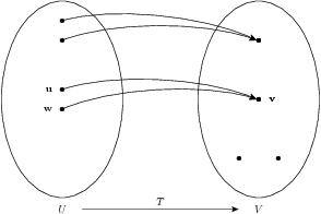
Here’s a cartoon of a non-injective linear transformation. Notice that the central feature of this cartoon is that T\left (u\right ) = v = T\left (w\right ). Even though this happens again with some unnamed vectors, it only takes one occurrence to destroy the possibility of injectivity. Note also that the two vectors displayed in the bottom of V have no bearing, either way, on the injectivity of T.
To show that a linear transformation is not injective, it is enough to find a single pair of inputs that get sent to the identical output, as in Example NIAQ. However, to show that a linear transformation is injective we must establish that this coincidence of outputs never occurs. Here is an example that shows how to establish this.
Example IAR
Injective, Archetype R
Archetype R is the linear transformation
|
T : {ℂ}^{5}\mathrel{↦}{ℂ}^{5},\quad T\left (\left [\array{
{x}_{1}
\cr
{x}_{2}
\cr
{x}_{3}
\cr
{x}_{4}
\cr
{x}_{5} } \right ]\right ) = \left [\array{
−65{x}_{1} + 128{x}_{2} + 10{x}_{3} − 262{x}_{4} + 40{x}_{5}
\cr
36{x}_{1} − 73{x}_{2} − {x}_{3} + 151{x}_{4} − 16{x}_{5}
\cr
−44{x}_{1} + 88{x}_{2} + 5{x}_{3} − 180{x}_{4} + 24{x}_{5}
\cr
34{x}_{1} − 68{x}_{2} − 3{x}_{3} + 140{x}_{4} − 18{x}_{5}
\cr
12{x}_{1} − 24{x}_{2} − {x}_{3} + 49{x}_{4} − 5{x}_{5} } \right ]
|
To establish that R is injective we must begin with the assumption that T\left (x\right ) = T\left (y\right ) and somehow arrive from this at the conclusion that x = y. Here we go,
Now we recognize that we have a homogeneous system of 5 equations in 5 variables (the terms {x}_{i} − {y}_{i} are the variables), so we row-reduce the coefficient matrix to
|
\left [\array{
\text{1}&0&0&0&0
\cr
0&\text{1}&0&0&0
\cr
0&0&\text{1}&0&0
\cr
0&0&0&\text{1}&0
\cr
0&0&0&0&\text{1} } \right ]
|
So the only solution is the trivial solution
and we conclude that indeed x = y. By Definition ILT, T is injective. ⊠
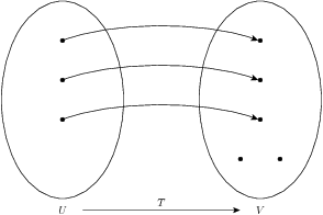
Here’s the cartoon for an injective linear transformation. It is meant to suggest that we never have two inputs associated with a single output. Again, the two lonely vectors at the bottom of V have no bearing either way on the injectivity of T.
Let’s now examine an injective linear transformation between abstract vector spaces.
Example IAV
Injective, Archetype V
Archetype V is defined by
|
T : {P}_{3}\mathrel{↦}{M}_{22},\quad T\left (a + bx + c{x}^{2} + d{x}^{3}\right ) = \left [\array{
a + b&a − 2c
\cr
d & b − d } \right ]
|
To establish that the linear transformation is injective, begin by supposing that two polynomial inputs yield the same output matrix,
|
T\left ({a}_{1} + {b}_{1}x + {c}_{1}{x}^{2} + {d}_{
1}{x}^{3}\right ) = T\left ({a}_{
2} + {b}_{2}x + {c}_{2}{x}^{2} + {d}_{
2}{x}^{3}\right )
|
Then
This single matrix equality translates to the homogeneous system of equations in the variables {a}_{i} − {b}_{i},
This system of equations can be rewritten as the matrix equation
|
\left [\array{
1&1& 0 & 0
\cr
1&0&−2& 0
\cr
0&0& 0 & 1
\cr
0&1& 0 &−1 } \right ]\left [\array{
({a}_{1} − {a}_{2})
\cr
({b}_{1} − {b}_{2})
\cr
({c}_{1} − {c}_{2})
\cr
({d}_{1} − {d}_{2}) } \right ] = \left [\array{
0
\cr
0
\cr
0
\cr
0 } \right ]
|
Since the coefficient matrix is nonsingular (check this) the only solution is trivial, i.e.
}
so the two inputs must be equal polynomials. By Definition ILT, T is injective. ⊠
For a linear transformation T : U\mathrel{↦}V , the kernel is a subset of the domain U. Informally, it is the set of all inputs that the transformation sends to the zero vector of the codomain. It will have some natural connections with the null space of a matrix, so we will keep the same notation, and if you think about your objects, then there should be little confusion. Here’s the careful definition.
Definition KLT
Kernel of a Linear Transformation
Suppose T : U\mathrel{↦}V
is a linear transformation. Then the kernel of
T is the
set
|
K\kern -1.95872pt \left (T\right ) = \left \{u ∈ U\mathrel{∣}T\left (u\right ) = 0\right \}
|
(This definition contains Notation KLT.) △
Notice that the kernel of T is just the preimage of 0, {T}^{−1}\left (0\right ) (Definition PI). Here’s an example.
Example NKAO
Nontrivial kernel, Archetype O
Archetype O is the linear transformation
|
T : {ℂ}^{3}\mathrel{↦}{ℂ}^{5},\quad T\left (\left [\array{
{x}_{1}
\cr
{x}_{2}
\cr
{x}_{3} } \right ]\right ) = \left [\array{
−{x}_{1} + {x}_{2} − 3{x}_{3}
\cr
−{x}_{1} + 2{x}_{2} − 4{x}_{3}
\cr
{x}_{1} + {x}_{2} + {x}_{3}
\cr
2{x}_{1} + 3{x}_{2} + {x}_{3}
\cr
{x}_{1} + 2{x}_{3} } \right ]
|
To determine the elements of {ℂ}^{3} in K\kern -1.95872pt \left (T\right ), find those vectors u such that T\left (u\right ) = 0, that is,
Vector equality (Definition CVE) leads us to a homogeneous system of 5 equations in the variables {u}_{i},
Row-reducing the coefficient matrix gives
|
\left [\array{
\text{1}&0& 2
\cr
0&\text{1}&−1
\cr
0&0& 0
\cr
0&0& 0
\cr
0&0& 0 } \right ]
|
The kernel of T is the set of solutions to this homogeneous system of equations, which by Theorem BNS can be expressed as
|
K\kern -1.95872pt \left (T\right ) = \left \langle \left \{\left [\array{
−2
\cr
1
\cr
1 } \right ]\right \}\right \rangle
|
We know that the span of a set of vectors is always a subspace (Theorem SSS), so the kernel computed in Example NKAO is also a subspace. This is no accident, the kernel of a linear transformation is always a subspace.
Theorem KLTS
Kernel of a Linear Transformation is a Subspace
Suppose that T : U\mathrel{↦}V
is a linear transformation. Then the kernel of
T,
K\kern -1.95872pt \left (T\right ), is a
subspace of U.
□
Proof We can apply the three-part test of Theorem TSS. First T\left ({0}_{U}\right ) = {0}_{V } by Theorem LTTZZ, so {0}_{U} ∈K\kern -1.95872pt \left (T\right ) and we know that the kernel is non-empty.
Suppose we assume that x,\kern 1.95872pt y ∈K\kern -1.95872pt \left (T\right ). Is x + y ∈K\kern -1.95872pt \left (T\right )?
This qualifies x + y for membership in K\kern -1.95872pt \left (T\right ). So we have additive closure.
Suppose we assume that α ∈ {ℂ}^{} and x ∈K\kern -1.95872pt \left (T\right ). Is αx ∈K\kern -1.95872pt \left (T\right )?
This qualifies αx for membership in K\kern -1.95872pt \left (T\right ). So we have scalar closure and Theorem TSS tells us that K\kern -1.95872pt \left (T\right ) is a subspace of U. ■
Let’s compute another kernel, now that we know in advance that it will be a subspace.
Example TKAP
Trivial kernel, Archetype P
Archetype P is the linear transformation
|
T : {ℂ}^{3}\mathrel{↦}{ℂ}^{5},\quad T\left (\left [\array{
{x}_{1}
\cr
{x}_{2}
\cr
{x}_{3} } \right ]\right ) = \left [\array{
−{x}_{1} + {x}_{2} + {x}_{3}
\cr
−{x}_{1} + 2{x}_{2} + 2{x}_{3}
\cr
{x}_{1} + {x}_{2} + 3{x}_{3}
\cr
2{x}_{1} + 3{x}_{2} + {x}_{3}
\cr
−2{x}_{1} + {x}_{2} + 3{x}_{3} } \right ]
|
To determine the elements of {ℂ}^{3} in K\kern -1.95872pt \left (T\right ), find those vectors u such that T\left (u\right ) = 0, that is,
Vector equality (Definition CVE) leads us to a homogeneous system of 5 equations in the variables {u}_{i},
Row-reducing the coefficient matrix gives
|
\left [\array{
\text{1}&0&0
\cr
0&\text{1}&0
\cr
0&0&\text{1}
\cr
0&0&0
\cr
0&0&0} \right ]
|
The kernel of T is the set of solutions to this homogeneous system of equations, which is simply the trivial solution u = 0, so
|
K\kern -1.95872pt \left (T\right ) = \left \{0\right \} = \left \langle \left \{\ \right \}\right \rangle
|
Our next theorem says that if a preimage is a non-empty set then we can construct it by picking any one element and adding on elements of the kernel.
Theorem KPI
Kernel and Pre-Image
Suppose T : U\mathrel{↦}V is a linear
transformation and v ∈ V .
If the preimage {T}^{−1}\left (v\right ) is
non-empty, and u ∈ {T}^{−1}\left (v\right )
then
|
{T}^{−1}\left (v\right ) = \left \{u + z\mathrel{∣}z ∈K\kern -1.95872pt \left (T\right )\right \} = u + K\kern -1.95872pt \left (T\right )
|
Proof Let M = \left \{u + z\mathrel{∣}z ∈K\kern -1.95872pt \left (T\right )\right \}. First, we show that M ⊆ {T}^{−1}\left (v\right ). Suppose that w ∈ M, so w has the form w = u + z, where z ∈K\kern -1.95872pt \left (T\right ). Then
which qualifies w for membership in the preimage of v, w ∈ {T}^{−1}\left (v\right ).
For the opposite inclusion, suppose x ∈ {T}^{−1}\left (v\right ). Then,
This qualifies x − u for membership in the kernel of T, K\kern -1.95872pt \left (T\right ). So there is a vector z ∈K\kern -1.95872pt \left (T\right ) such that x − u = z. Rearranging this equation gives x = u + z and so x ∈ M. So {T}^{−1}\left (v\right ) ⊆ M and we see that M = {T}^{−1}\left (v\right ), as desired. ■
This theorem, and its proof, should remind you very much of Theorem PSPHS. Additionally, you might go back and review Example SPIAS. Can you tell now which is the only preimage to be a subspace?
The next theorem is one we will cite frequently, as it characterizes injections by the size of the kernel.
Theorem KILT
Kernel of an Injective Linear Transformation
Suppose that T : U\mathrel{↦}V is a linear
transformation. Then T is injective
if and only if the kernel of T
is trivial, K\kern -1.95872pt \left (T\right ) = \left \{0\right \}.
□
Proof ( ⇒) We assume T is injective and we need to establish that two sets are equal (Definition SE). Since the kernel is a subspace (Theorem KLTS), \left \{0\right \} ⊆K\kern -1.95872pt \left (T\right ). To establish the opposite inclusion, suppose x ∈K\kern -1.95872pt \left (T\right ).
We can apply Definition ILT to conclude that x = 0. Therefore K\kern -1.95872pt \left (T\right ) ⊆\left \{0\right \} and by Definition SE, K\kern -1.95872pt \left (T\right ) = \left \{0\right \}.
( ⇐) To establish that T is injective, appeal to Definition ILT and begin with the assumption that T\left (x\right ) = T\left (y\right ). Then
So x − y ∈K\kern -1.95872pt \left (T\right ) by Definition KLT and with the hypothesis that the kernel is trivial we conclude that x − y = 0. Then
thus establishing that T is injective by Definition ILT. ■
Example NIAQR
Not injective, Archetype Q, revisited
We are now in a position to revisit our first example in this section,
Example NIAQ. In that example, we showed that Archetype Q is not injective by
constructing two vectors, which when used to evaluate the linear transformation
provided the same output, thus violating Definition ILT. Just where did those
two vectors come from?
The key is the vector
|
z = \left [\array{
3
\cr
4
\cr
1
\cr
3
\cr
3 } \right ]
|
which you can check is an element of K\kern -1.95872pt \left (T\right ) for Archetype Q. Choose a vector x at random, and then compute y = x + z (verify this computation back in Example NIAQ). Then
Whenever the kernel of a linear transformation is non-trivial, we can employ this device and conclude that the linear transformation is not injective. This is another way of viewing Theorem KILT. For an injective linear transformation, the kernel is trivial and our only choice for z is the zero vector, which will not help us create two different inputs for T that yield identical outputs. For every one of the archetypes that is not injective, there is an example presented of exactly this form. ⊠
Example NIAO
Not injective, Archetype O
In Example NKAO the kernel of Archetype O was determined to be
|
\left \langle \left \{\left [\array{
−2
\cr
1
\cr
1 } \right ]\right \}\right \rangle
|
a subspace of {ℂ}^{3} with dimension 1. Since the kernel is not trivial, Theorem KILT tells us that T is not injective. ⊠
Example IAP
Injective, Archetype P
In Example TKAP it was shown that the linear transformation
in Archetype P has a trivial kernel. So by Theorem KILT,
T is
injective. ⊠
There is a connection between injective linear transformations and linearly independent sets that we will make precise in the next two theorems. However, more informally, we can get a feel for this connection when we think about how each property is defined. A set of vectors is linearly independent if the only relation of linear dependence is the trivial one. A linear transformation is injective if the only way two input vectors can produce the same output is if the trivial way, when both input vectors are equal.
Theorem ILTLI
Injective Linear Transformations and Linear Independence
Suppose that T : U\mathrel{↦}V
is an injective linear transformation and
S = \left \{{u}_{1},\kern 1.95872pt {u}_{2},\kern 1.95872pt {u}_{3},\kern 1.95872pt \mathop{\mathop{…}},\kern 1.95872pt {u}_{t}\right \} is a linearly
independent subset of U.
Then R = \left \{T\left ({u}_{1}\right ),\kern 1.95872pt T\left ({u}_{2}\right ),\kern 1.95872pt T\left ({u}_{3}\right ),\kern 1.95872pt \mathop{\mathop{…}},\kern 1.95872pt T\left ({u}_{t}\right )\right \} is a linearly
independent subset of V .
□
Proof Begin with a relation of linear dependence on R (Definition RLD, Definition LI),
Since this is a relation of linear dependence on the linearly independent set S, we can conclude that
and this establishes that R is a linearly independent set. ■
Theorem ILTB
Injective Linear Transformations and Bases
Suppose that T : U\mathrel{↦}V is a linear
transformation and B = \left \{{u}_{1},\kern 1.95872pt {u}_{2},\kern 1.95872pt {u}_{3},\kern 1.95872pt \mathop{\mathop{…}},\kern 1.95872pt {u}_{m}\right \}
is a basis of U. Then
T is injective if and
only if C = \left \{T\left ({u}_{1}\right ),\kern 1.95872pt T\left ({u}_{2}\right ),\kern 1.95872pt T\left ({u}_{3}\right ),\kern 1.95872pt \mathop{\mathop{…}},\kern 1.95872pt T\left ({u}_{m}\right )\right \} is a linearly
independent subset of V .
□
Proof ( ⇒) Assume T is injective. Since B is a basis, we know B is linearly independent (Definition B). Then Theorem ILTLI says that C is a linearly independent subset of V .
( ⇐) Assume that C is linearly independent. To establish that T is injective, we will show that the kernel of T is trivial (Theorem KILT). Suppose that u ∈K\kern -1.95872pt \left (T\right ). As an element of U, we can write u as a linear combination of the basis vectors in B (uniquely). So there are are scalars, {a}_{1},\kern 1.95872pt {a}_{2},\kern 1.95872pt {a}_{3},\kern 1.95872pt \mathop{\mathop{…}},\kern 1.95872pt {a}_{m}, such that
|
u = {a}_{1}{u}_{1} + {a}_{2}{u}_{2} + {a}_{3}{u}_{3} + \mathrel{⋯} + {a}_{m}{u}_{m}
|
Then,
This is a relation of linear dependence (Definition RLD) on the linearly independent set C, so the scalars are all zero: {a}_{1} = {a}_{2} = {a}_{3} = \mathrel{⋯} = {a}_{m} = 0. Then
Since u was chosen as an arbitrary vector from K\kern -1.95872pt \left (T\right ), we have K\kern -1.95872pt \left (T\right ) = \left \{0\right \} and Theorem KILT tells us that T is injective. ■
Theorem ILTD
Injective Linear Transformations and Dimension
Suppose that T : U\mathrel{↦}V is an injective
linear transformation. Then \mathop{ dim}\nolimits \left (U\right ) ≤\mathop{ dim}\nolimits \left (V \right ).
□
Proof Suppose to the contrary that m =\mathop{ dim}\nolimits \left (U\right ) >\mathop{ dim}\nolimits \left (V \right ) = t. Let B be a basis of U, which will then contain m vectors. Apply T to each element of B to form a set C that is a subset of V . By Theorem ILTB, C is linearly independent and therefore must contain m distinct vectors. So we have found a set of m linearly independent vectors in V , a vector space of dimension t, with m > t. However, this contradicts Theorem G, so our assumption is false and \mathop{ dim}\nolimits \left (U\right ) ≤\mathop{ dim}\nolimits \left (V \right ). ■
Example NIDAU
Not injective by dimension, Archetype U
The linear transformation in Archetype U is
|
T : {M}_{23}\mathrel{↦}{ℂ}^{4},\quad T\left (\left [\array{
a&b&c
\cr
d&e&f} \right ]\right ) = \left [\array{
a + 2b + 12c − 3d + e + 6f
\cr
2a − b − c + d − 11f
\cr
a + b + 7c + 2d + e − 3f
\cr
a + 2b + 12c + 5e − 5f } \right ]
|
Since \mathop{ dim}\nolimits \left ({M}_{23}\right ) = 6 > 4 =\mathop{ dim}\nolimits \left ({ℂ}^{4}\right ), T cannot be injective for then T would violate Theorem ILTD. ⊠
Notice that the previous example made no use of the actual formula defining the function. Merely a comparison of the dimensions of the domain and codomain are enough to conclude that the linear transformation is not injective. Archetype M and Archetype N are two more examples of linear transformations that have “big” domains and “small” codomains, resulting in “collisions” of outputs and thus are non-injective linear transformations.
In Subsection LT.NLTFO we saw how to combine linear transformations to build new linear transformations, specifically, how to build the composition of two linear transformations (Definition LTC). It will be useful later to know that the composition of injective linear transformations is again injective, so we prove that here.
Theorem CILTI
Composition of Injective Linear Transformations is Injective
Suppose that T : U\mathrel{↦}V
and S : V \mathrel{↦}W
are injective linear transformations. Then
(S ∘ T): U\mathrel{↦}W is an injective linear
transformation. □
Proof That the composition is a linear transformation was established in Theorem CLTLT, so we need only establish that the composition is injective. Applying Definition ILT, choose x, y from U. Then if \left (S ∘ T\right )\left (x\right ) = \left (S ∘ T\right )\left (y\right ),
C10 Each archetype below is a linear transformation. Compute the kernel
for each.
Archetype M
Archetype N
Archetype O
Archetype P
Archetype Q
Archetype R
Archetype S
Archetype T
Archetype U
Archetype V
Archetype W
Archetype X
Contributed by Robert Beezer
C20 The linear transformation T : {ℂ}^{4}\mathrel{↦}{ℂ}^{3} is not injective. Find two inputs x,\kern 1.95872pt y ∈ {ℂ}^{4} that yield the same output (that is T\left (x\right ) = T\left (y\right )).
|
T\left (\left [\array{
{x}_{1}
\cr
{x}_{2}
\cr
{x}_{3}
\cr
{x}_{4} } \right ]\right ) = \left [\array{
2{x}_{1} + {x}_{2} + {x}_{3}
\cr
−{x}_{1} + 3{x}_{2} + {x}_{3} − {x}_{4}
\cr
3{x}_{1} + {x}_{2} + 2{x}_{3} − 2{x}_{4} } \right ]
|
Contributed by Robert Beezer Solution [1421]
C25 Define the linear transformation
|
T : {ℂ}^{3}\mathrel{↦}{ℂ}^{2},\quad T\left (\left [\array{
{x}_{1}
\cr
{x}_{2}
\cr
{x}_{3} } \right ]\right ) = \left [\array{
2{x}_{1} − {x}_{2} + 5{x}_{3}
\cr
−4{x}_{1} + 2{x}_{2} − 10{x}_{3} } \right ]
|
Find a basis for the kernel of T,
K\kern -1.95872pt \left (T\right ). Is
T
injective?
Contributed by Robert Beezer Solution [1424]
C40 Show that the linear transformation R is not injective by finding two different elements of the domain, x and y, such that R\left (x\right ) = R\left (y\right ). ({S}_{22} is the vector space of symmetric 2 × 2 matrices.)
|
R: {S}_{22}\mathrel{↦}{P}_{1}\quad R\left (\left [\array{
a&b
\cr
b&c } \right ]\right ) = (2a−b+c)+(a+b+2c)x
|
Contributed by Robert Beezer Solution [1425]
T10 Suppose T : U\mathrel{↦}V
is a linear transformation. For which vectors
v ∈ V is
{T}^{−1}\left (v\right ) a subspace
of U?
Contributed by Robert Beezer
T15 Suppose that that T : U\mathrel{↦}V and S : V \mathrel{↦}W are linear transformations. Prove the following relationship between null spaces.
|
K\kern -1.95872pt \left (T\right ) ⊆K\kern -1.95872pt \left (S ∘ T\right )
|
Contributed by Robert Beezer Solution [1427]
T20 Suppose that A is an m × n matrix. Define the linear transformation T by
|
T : {ℂ}^{n}\mathrel{↦}{ℂ}^{m},\quad T\left (x\right ) = Ax
|
Prove that the kernel of T
equals the null space of A,
K\kern -1.95872pt \left (T\right ) = N\kern -1.95872pt \left (A\right ).
Contributed by Andy Zimmer Solution [1427]
C20 Contributed by Robert Beezer Statement [1417]
A linear transformation that is not injective will have a non-trivial
kernel (Theorem KILT), and this is the key to finding the desired
inputs. We need one non-trivial element of the kernel, so suppose that
z ∈ {ℂ}^{4} is an
element of the kernel,
|
\left [\array{
0
\cr
0
\cr
0 } \right ] = 0 = T\left (z\right ) = \left [\array{
2{z}_{1} + {z}_{2} + {z}_{3}
\cr
−{z}_{1} + 3{z}_{2} + {z}_{3} − {z}_{4}
\cr
3{z}_{1} + {z}_{2} + 2{z}_{3} − 2{z}_{4} } \right ]
|
Vector equality Definition CVE leads to the homogeneous system of three equations in four variables,
The coefficient matrix of this system row-reduces as
|
\left [\array{
2 &1&1& 0
\cr
−1&3&1&−1
\cr
3 &1&2&−2 } \right ]\mathop{\longrightarrow}\limits_{}^{\text{RREF}}\left [\array{
\text{1}&0&0& 1
\cr
0&\text{1}&0& 1
\cr
0&0&\text{1}&−3 } \right ]
|
From this we can find a solution (we only need one), that is an element of K\kern -1.95872pt \left (T\right ),
|
z = \left [\array{
−1
\cr
−1
\cr
3
\cr
1 } \right ]
|
Now, we choose a vector x at random and set y = x + z,
and you can check that
|
T\left (x\right ) = \left [\array{
11
\cr
13
\cr
21 } \right ] = T\left (y\right )
|
A quicker solution is to take two elements of the kernel (in this case, scalar multiples of z) which both get sent to 0 by T. Quicker yet, take 0 and z as x and y, which also both get sent to 0 by T.
C25 Contributed by Robert Beezer Statement [1418]
To find the kernel, we require all x ∈ {ℂ}^{3}
such that T\left (x\right ) = 0.
This condition is
|
\left [\array{
2{x}_{1} − {x}_{2} + 5{x}_{3}
\cr
−4{x}_{1} + 2{x}_{2} − 10{x}_{3} } \right ] = \left [\array{
0
\cr
0 } \right ]
|
This leads to a homogeneous system of two linear equations in three variables, whose coefficient matrix row-reduces to
|
\left [\array{
\text{1}&−{1\over
2}&{5\over
2}
\cr
0& 0 &0 } \right ]
|
With two free variables Theorem BNS yields the basis for the null space
|
\left \{\left [\array{
−{5\over
2}
\cr
0
\cr
1 } \right ],\kern 1.95872pt \left [\array{
{1\over
2}
\cr
1
\cr
0 } \right ]\right \}
|
With n\left (T\right )\mathrel{≠}0, K\kern -1.95872pt \left (T\right )\mathrel{≠}\left \{0\right \}, so Theorem KILT says T is not injective.
C40 Contributed by Robert Beezer Statement [1418]
We choose x
to be any vector we like. A particularly cocky choice would be to choose
x = 0, but
we will instead choose
|
x = \left [\array{
2 &−1
\cr
−1& 4 } \right ]
|
Then R\left (x\right ) = 9 + 9x. Now compute the kernel of R, which by Theorem KILT we expect to be nontrivial. Setting R\left (\left [\array{ a&b \cr b&c } \right ]\right )equalto the zero vector, 0 = 0 + 0x, and equating coefficients leads to a homogeneous system of equations. Row-reducing the coefficient matrix of this system will allow us to determine the values of a, b and c that create elements of the null space of R,
|
\left [\array{
2&−1&1
\cr
1& 1 &2 } \right ]\mathop{\longrightarrow}\limits_{}^{\text{RREF}}\left [\array{
\text{1}&0&1
\cr
0&\text{1}&1} \right ]
|
We only need a single element of the null space of this coefficient matrix, so we will not compute a precise description of the whole null space. Instead, choose the free variable c = 2. Then
|
z = \left [\array{
−2&−2
\cr
−2& 2 } \right ]
|
is the corresponding element of the kernel. We compute the desired y as
|
y = x+z = \left [\array{
2 &−1
\cr
−1& 4 } \right ]+\left [\array{
−2&−2
\cr
−2& 2 } \right ] = \left [\array{
0 &−3
\cr
−3& 6 } \right ]
|
Then check that R\left (y\right ) = 9 + 9x.
T15 Contributed by Robert Beezer Statement [1419]
We are asked to prove that K\kern -1.95872pt \left (T\right )
is a subset of K\kern -1.95872pt \left (S ∘ T\right ). Employing
Definition SSET, choose x ∈K\kern -1.95872pt \left (T\right ).
Then we know that T\left (x\right ) = 0.
So
This qualifies x for membership in K\kern -1.95872pt \left (S ∘ T\right ).
T20 Contributed by Andy Zimmer Statement [1419]
This is an equality of sets, so we want to establish two subset conditions
(Definition SE).
First, show N\kern -1.95872pt \left (A\right ) ⊆K\kern -1.95872pt \left (T\right ). Choose x ∈N\kern -1.95872pt \left (A\right ). Check to see if x ∈K\kern -1.95872pt \left (T\right ),
So by Definition KLT, x ∈K\kern -1.95872pt \left (T\right ) and thus N\kern -1.95872pt \left (A\right ) ⊆N\kern -1.95872pt \left (T\right ).
Now, show K\kern -1.95872pt \left (T\right ) ⊆N\kern -1.95872pt \left (A\right ). Choose x ∈K\kern -1.95872pt \left (T\right ). Check to see if x ∈N\kern -1.95872pt \left (A\right ),
So by Definition NSM, x ∈N\kern -1.95872pt \left (A\right ) and thus N\kern -1.95872pt \left (T\right ) ⊆N\kern -1.95872pt \left (A\right ).