Section4.2Generalized Quadrangles
A generalized quadrangle is an incidence structure of points and lines such that
- Any two points lie on at most one line.
- If the point \(x\) is off the line \(\ell\), then there is a unique point on \(\ell\) collinear with \(x\).
These axioms are self-dual, and therefore the incidence structure dual to a \(GQ\) is again a \(GQ\).
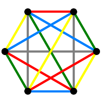
The smallest interesting example has as points the 15 edges of \(K_6\) and as lines the 15 1-factors of \(K_6\); each edge is incident with the three 1-factors that contain it. A \(GQ\) is thick if each point is on at least three lines and each line contains at least three points. If a \(GQ\) is thick then it is point and line regular, this means there are integers \(s\) and \(t\) such that each point lies on exactly \(t+1\) lines and each line contains exactly \(s+1\) points. Our example above is a \(GQ(2,2)\), traditionally denoted by \(W(2)\).
Associated to an incidence structure we have a point graph, a line graph and an incidence graph. For \(W(2)\) the point and line graphs are isomorphic to \(L(K_6)\) (which is very easy to check); the incidence graph is a bipartite cubic graph on 30 vertices with diameter four and girth eight. It is known as Tutte's 8-cage. For a thick \(GQ\), both the point and line graphs are strongly regular.
We describe how to construct a family of \(GQ\)'s denoted by \(W(q)\), where \(q\) is a primes power. We will accompany the description with the code for \(W(3)\).
Let \(V\) be the vector space of dimension four over \(GF(q)\). Its 1-dimensional subspaces will be the points of our generalized quadrangle. To define the lines we want a non-degenerate alternating form on \(V\); this is given by an invertible matrix \(S\) with diagonal entries zero such that \(S+S^T=0\). (So if \(q\) is odd, then \(S\) is skew symmetric; if \(q\) is even it's symmetric with zero diagonal.) A subspace \(U\) of \(V\) is isotropic if
Time for some actual work. We define our form:
and create our points and lines:
Two points \(u\) and \(v\) are collinear if \(\beta(u,v)=0\). Two lines \(L\) and \(M\) are incident if
or if they are not equal and
Elements of our vector space \(V\) are "mutable", so not hashable, and therefore cannot be used as vertices of a graph. This is easily circumvented:
We can check that \(W3\) is connected and regular, and that it has exactly three eigenvalues (obvious in the factored characteristic polynomial):
The lines of the \(GQ\) correspond to the cliques of maximal size, which we can find by
You can check that the number of cliques is correct. We get the point graph of the dual \(GQ\) by
As expected \(W3d\) is not isomorphic to \(W3\), but it is strongly regular with the same parameters.
but it is strongly regular
and it has the same characteristic polynomial (and hence the same parameters).