Section6.1Projective Plane of Order 4
A projective plane of order \(n\) is a \(2-(n^2+n+1, n+1, 1)\) design. Such a design is therefore a collection of sets (called blocks), each of size \(n+1\), chosen from a universal set of size \(n^2+n+1\), with the property that any \(2\) elements chosen from the universal set is contained in exactly \(1\) of the blocks.
As a finite geometry a projective plane of order \(n\) is a set of points and lines, together with an incidence relation, such that:
- Exactly one line passes through any two points.
- Any two lines pass through exactly one common point.
- Every point has exactly \(n+1\) lines pasing through the point.
- Every line passes through exactly \(n+1\) points.
Here the notion of a line “passing through” a point is more precisely given by the incidence relation. One common such relation is that lines are sets of points, and a point and line are incident if the point is an element of the line.
A finite projective plane of order 4 is equivalent to a set of three mutually orthogonal Latin Squares (see Chapter 12 of Combinatorial Theory, by Marshall Hall, Jr). The impossibility of the projective plane of order \(10\) was only settled in the late 1980s by Clement Lam.
We first need some of the objects we computed in Chapter 5, so evaluate the next cell to get started.
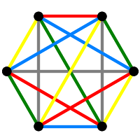
We will build a design from our factorizations by first building a graph that describes an incidence relation. The points of the geometry will be the six vertices of \(K_6\) together with the fifteen factors of \(K_6\). The lines of the geometry will be the fifteen edges of \(K_6\) along with the six factorizations of \(K_6\). So we have \(21\) points and \(21\) lines. The graph will be bipartite with points in one set of the bipartition and lines in the other set. A vertex will be incident to an edge which contains it, a factor will be incident to an edge if the factor contains the edge, and a factor will be incident to factorization which contains it.
The resulting biparite graph is regular of degree \(5\) on \(42\) vertices with girth \(6\).
We can relabel the vertices of a copy of the graph, and then have Sage recognize the bipartite structure before producing a drawing. First, create the same dictionaries of names we used in Chapter 5.
If we call Sage's relabeling function with no arguments, the points will be labeled with the integers \(0\) to \(20\) and the lines will be labeled with the integers \(21\) to \(41\). We can create the blocks of a block design by creating lists of the points on each line.
So the parameters are those of a \(2-(21, 5, 1)\) design, a projective plane of order \(4\).
We can list all of the \(21\) blocks, if we wish.
Notice that this section is made possible by the arithmetic: \(6+15=21=4^2+4+1\).