\( \newcommand\al{\alpha} \newcommand\be{\beta} \newcommand\de{\delta} \newcommand\De{\Delta} \newcommand\eps{\epsilon} \newcommand\ga{\gamma} \newcommand\Ga{\Gamma} \newcommand\ka{\kappa} \newcommand\la{\lambda} \newcommand\La{\Lambda} \newcommand\om{\omega} \newcommand\Om{\Omega} \newcommand\sg{\sigma} \newcommand\Sg{\Sigma} \renewcommand\th{\theta} %--- Latex uses \th for a Norse character \newcommand\Th{\Theta} \newcommand\vphi{\varphi} % % some calligraphy % \newcommand\cA{{\mathcal A}} \newcommand\cB{{\mathcal B}} \newcommand\cC{{\mathcal C}} \newcommand\cD{{\mathcal D}} \newcommand\cE{{\mathcal E}} \newcommand\cF{{\mathcal F}} \newcommand\cG{{\mathcal G}} \newcommand\cH{{\mathcal H}} \newcommand\cI{{\mathcal I}} \newcommand\cJ{{\mathcal J}} \newcommand\cK{{\mathcal K}} \newcommand\cL{{\mathcal L}} \newcommand\cM{{\mathcal M}} \newcommand\cN{{\mathcal N}} \newcommand\cO{{\mathcal O}} \newcommand\cP{{\mathcal P}} \newcommand\cQ{{\mathcal Q}} \newcommand\cR{{\mathcal R}} \newcommand\cS{{\mathcal S}} \newcommand\cT{{\mathcal T}} \newcommand\cU{{\mathcal U}} \newcommand\cV{{\mathcal V}} % % fields and rings (and a semigroup) % \newcommand\cx{{\mathbb C}}% complexes \newcommand\fld{{\mathbb F}} \newcommand\flde{{\mathbb E}} \newcommand\ints{{\mathbb Z}} \newcommand\nn{{\mathbb N}}%non-negative integers \newcommand\re{{\mathbb R}}%reals \newcommand\rats{{\mathbb Q}} % % the really useful stuff % \newcommand\comp[1]{{\mkern2mu\overline{\mkern-2mu#1}}} \newcommand\diff{\mathbin{\mkern-1.5mu\setminus\mkern-1.5mu}}% for \setminus \newcommand\res{\mathbin{\mkern-2.0mu\restriction\mkern-2.0mu}} \newcommand\sbs{\subseteq} \newcommand\sps{\supseteq} \newcommand\seq[3]{#1_{#2},\ldots,#1_{#3}} \DeclareMathOperator{\supp}{supp} \DeclareMathOperator{\im}{im} \DeclareMathOperator{\row}{row} \newcommand\pmat[1]{\begin{pmatrix} #1 \end{pmatrix}} \newcommand\cprod{\mathbin{\square}} \newcommand\gbin[2]{\genfrac{[}{]}{0pt}{}{#1}{#2}} % % matrix theory % \newcommand\ip[2]{\langle#1,#2\rangle} \newcommand\one{{\bf1}} \DeclareMathOperator{\rk}{rk} \DeclareMathOperator{\tr}{tr} \DeclareMathOperator{\col}{col} \newcommand\mat[3]{\mathrm{Mat}_{#1\times #2}(#3)} \newcommand\sm[3]{\sum_{#1=#2}^{#3}} % % some group theory % \newcommand\aut[1]{{\rm Aut}(#1)} \newcommand\fx[1]{{\rm fix}(#1)}% ch2 \newcommand\grp[1]{\langle #1\rangle} \newcommand\nrml{\vartriangleleft} \newcommand\nrmleq{\trianglelefteq} \DeclareMathOperator{\Sym}{Sym} \newcommand\sym[1]{\Sym(#1)} \DeclareMathOperator{\Alt}{Alt} \newcommand\alt[1]{\Alt(#1)} \)

Section1.3Basics

Sage comes with many graphs preinstalled. Thus the command

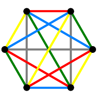
sets \(K\) equal to the complete graph on 5 vertices. Now K.show() produces a drawing of the graph in a separate window.

The command

displays the vertices of our graph and

displays the edges. To avoid the empty labels, try

The command K.degree() produces a list of the vertex degrees, while K.deg(u) gives the degree of the vertex \(u\). Further K[i] returns the neighbors of \(i\) in \(K\). If your graph is regular (K.is_regular() returns True) then its valency is given by

There are many built-in graphs in Sage. Thus:

gives us the cycle on 8 vertices. To get the list of possible graphs, type graphs. at the prompt, followed by a tab. (That's 8 keypresses—6 letters, a period and a tab.)

There are many graph operations we can use. We can get the complement of our cycle by

and its line graph by

Of course a cycle is isomorphic to its line graph, which we can verify:

Another way to verify that \(LC\) is the cycle \(C_8\) is to verify that it is connected

and that it is regular of degree two

Sage supplies the Petersen graph

and we can verify this is correct by computing its diameter, girth and the number of vertices since these three properties characterize the graph.

In practice it is very important to check that any graph you construct is the one you wanted. It may be hard to prove that your graph is correct, but simple checks can still be useful. One common source of error is an incomplete understanding of the commands you use. For example

produces a graph on three vertices!

I should have used K2.disjoint_union(K3).