Section5.2Factorizations of \(K_6\)
A factorization, or more precisely a \(1\)-factorization, is a partition of the edge set of a graph into \(1\)-factors. For \(K_6\) this is a partition of the \({6\choose 2}=15\) edges into \(5\) factors with \(3\) edges each.
We will see that \(K_6\) has six distinct factorizations, each isomorphic to the other. Furthermore, each factor is contained in exactly two of these factorizations, and any pair of factorizations have exactly one factor in common. So given a factor we can determine a pair of factorizations and given a pair of factorizations we can determine a factor. These observations will be critical in the following, especially the section on duality. These claims can be verified analytically — we will instead use Sage experimentally.
Begin by evaluating the next cell, which will re-create the factors of \(K_6\) for use in this section.
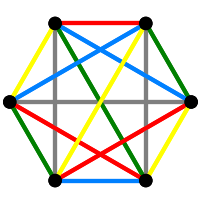
We begin by employing a graph to help us find the factorizations. The vertices of the graph are the factors of \(K_6\), and we join two vertices if the factors are disjoint. Then a factorization of \(K_6\) is a clique of size \(5\) in this graph, and there is no possibility of any larger clique because the edge set is exhausted by \(5\) disjoint factors. So factorizations of \(K_6\) are maximal cliques in this graph, which we record as Sage sets.
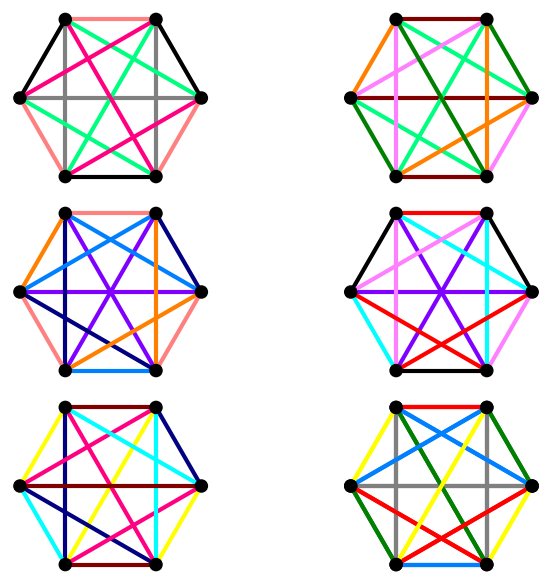
To visualize factorizations, it helps to look at a drawing of \(K_6\) with edges colored according to the factor they belong to. We build an ad-hoc set of fifteen contrasting colors as RGB triples and assign them to the factors with a Python dictionary. We will consistently use this color assignment in the remainder.
We now build and draw a copy of \(K_6\) for each factorization, using the provided color for the edges of each factor in the factorization. We will employ the one_K6_graphic() function twice, so be sure to execute it first. We exercise some of the graphics primitives for a little more control over the design of our diagrams.
We made two claims above about factors and factorizations: any single factor is contained in exactly two factorizations, and any two factorizations share a single common factor. For each factor, we form a list of factorizations containing that factor, and then simply check that the size (length) of that list is \(2\) in each case. Then we examine all pairs of factorizations, determining the size of the set of common factors for each pair.
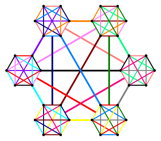
As any two factorizations share a single factor, we can make the \(6\) factorizations the vertices of a graph, add every possible edge (a complete graph) and color each edge with the color of the factor shared by the two factorizations at the endpoints.