\( \newcommand\al{\alpha} \newcommand\be{\beta} \newcommand\de{\delta} \newcommand\De{\Delta} \newcommand\eps{\epsilon} \newcommand\ga{\gamma} \newcommand\Ga{\Gamma} \newcommand\ka{\kappa} \newcommand\la{\lambda} \newcommand\La{\Lambda} \newcommand\om{\omega} \newcommand\Om{\Omega} \newcommand\sg{\sigma} \newcommand\Sg{\Sigma} \renewcommand\th{\theta} %--- Latex uses \th for a Norse character \newcommand\Th{\Theta} \newcommand\vphi{\varphi} % % some calligraphy % \newcommand\cA{{\mathcal A}} \newcommand\cB{{\mathcal B}} \newcommand\cC{{\mathcal C}} \newcommand\cD{{\mathcal D}} \newcommand\cE{{\mathcal E}} \newcommand\cF{{\mathcal F}} \newcommand\cG{{\mathcal G}} \newcommand\cH{{\mathcal H}} \newcommand\cI{{\mathcal I}} \newcommand\cJ{{\mathcal J}} \newcommand\cK{{\mathcal K}} \newcommand\cL{{\mathcal L}} \newcommand\cM{{\mathcal M}} \newcommand\cN{{\mathcal N}} \newcommand\cO{{\mathcal O}} \newcommand\cP{{\mathcal P}} \newcommand\cQ{{\mathcal Q}} \newcommand\cR{{\mathcal R}} \newcommand\cS{{\mathcal S}} \newcommand\cT{{\mathcal T}} \newcommand\cU{{\mathcal U}} \newcommand\cV{{\mathcal V}} % % fields and rings (and a semigroup) % \newcommand\cx{{\mathbb C}}% complexes \newcommand\fld{{\mathbb F}} \newcommand\flde{{\mathbb E}} \newcommand\ints{{\mathbb Z}} \newcommand\nn{{\mathbb N}}%non-negative integers \newcommand\re{{\mathbb R}}%reals \newcommand\rats{{\mathbb Q}} % % the really useful stuff % \newcommand\comp[1]{{\mkern2mu\overline{\mkern-2mu#1}}} \newcommand\diff{\mathbin{\mkern-1.5mu\setminus\mkern-1.5mu}}% for \setminus \newcommand\res{\mathbin{\mkern-2.0mu\restriction\mkern-2.0mu}} \newcommand\sbs{\subseteq} \newcommand\sps{\supseteq} \newcommand\seq[3]{#1_{#2},\ldots,#1_{#3}} \DeclareMathOperator{\supp}{supp} \DeclareMathOperator{\im}{im} \DeclareMathOperator{\row}{row} \newcommand\pmat[1]{\begin{pmatrix} #1 \end{pmatrix}} \newcommand\cprod{\mathbin{\square}} \newcommand\gbin[2]{\genfrac{[}{]}{0pt}{}{#1}{#2}} % % matrix theory % \newcommand\ip[2]{\langle#1,#2\rangle} \newcommand\one{{\bf1}} \DeclareMathOperator{\rk}{rk} \DeclareMathOperator{\tr}{tr} \DeclareMathOperator{\col}{col} \newcommand\mat[3]{\mathrm{Mat}_{#1\times #2}(#3)} \newcommand\sm[3]{\sum_{#1=#2}^{#3}} % % some group theory % \newcommand\aut[1]{{\rm Aut}(#1)} \newcommand\fx[1]{{\rm fix}(#1)}% ch2 \newcommand\grp[1]{\langle #1\rangle} \newcommand\nrml{\vartriangleleft} \newcommand\nrmleq{\trianglelefteq} \DeclareMathOperator{\Sym}{Sym} \newcommand\sym[1]{\Sym(#1)} \DeclareMathOperator{\Alt}{Alt} \newcommand\alt[1]{\Alt(#1)} \)

Section6.2Hoffman-Singleton Graph

The Hoffman-Singleton Graph is an amazing structure, which can be created many different ways. It is best known as a Moore graph: regular of degree \(7\) with odd girth \(5\), on \(50\) vertices, which is the minimum conceivable number.

We first need some of the objects we computed in Chapter 5, so evaluate the next cell to get started.

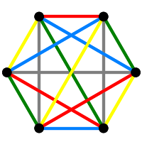
Our construction begins with two new vertices, which Cameron and van Lint call “zero” and “infinity” — we will shorten the label on the latter to simply “inf.” Zero and infinity will be adjacent to each other, zero will be adjacent to each vertex of \(K_6\) and infinity will be adjacent to each factorization of \(K_6\).

We have \(14\) vertices in our graph so far, we get another \(36\) from the Cartesian product of the set of \(6\) \(K_6\) vertices with the set of \(6\) factorizations. Each pair is joined to the \(K_6\) vertex of the pair and the factorization in the pair. At this point the vertices from the Cartesian product have just degree \(2\), the other vertices have reached degree \(7\).

Among vertices of the Cartesian product a pair \((a, x)\) is adjacent to the pair \((b, y)\) if \(x\) and \(y\) are different factorizations and the edge \(\{a, b\}\) is contained in the factor common to \(x\) and \(y\). (Recall that every pair of factorizations have a single factor in common.)

Construction complete, we can check that the graph has the requisite properties to be the Moore graph of degree \(7\) and girth \(5\).

Since these properties are enough to characterize the graph, we know we have it. However, we will let Sage do a brutish check. Our graph will not plot very nicely, while the implementation of the graph in Sage has a very novel feature. Each time you create the Hoffman-Singleton graph, you get a different layout, always displaying some of the inherent symmetry. So you can run the construct-and-plot command below repeatedly to experience different layouts.

Notice that this section is made possible by the arithmetic: \(50 = 2 + 6 + 6 + 6\cdot 6\).