Shortly after we built the six factorizations of \(K_6\), we created a graphic which was another version of \(K_6\) with factorizations as vertices and factors labeling (coloring) edges. This was possible, since as we also demonstrated above, every pair of factorizations have a single factor in common, and each factor is contained in exactly two factorizations. This version of \(K_6\) is “dual” to the original \(K_6\), as we will describe in this section. We need to create again the factorizations from previous sections of this chapter.
Build a graph, \(Q\), whose vertices are the factorizations of \(K_6\), with two vertices adjacent if the factorizations have a factor in common. The code below is a bit overblown, as we expect this graph to be isomorphic to \(K_6\). To emphasize the situation, we will label the vertices of \(Q\) (factorizations) by using names, uppercase letters from the end of the alphabet.
You can see it, but we will let Sage do the work for us.
By construction, the factorizations of \(K_6\) are the vertices of \(Q\). The factors of \(K_6\), by the discussion above, are in a bijective correspondence with the edges of \(Q\) (pairs of factorizations). We illustrate these ideas with functions that accept the factorizations and factors of \(K_6\) (respectively) and return the vertices and edges of \(Q\). To emphasize the nature of the situation, the trivial function that takes factorizations to vertices will return the factorization names provided by the Python dictionary factorization_names. We test these functions exhaustively. Also, notice how the second function employs the first.
Now we describe a natural bijection between edges of \(K_6\) and factors of \(Q\). Given an edge of \(K_6\), there remain four vertices not incident to this edge. The subgraph induced by these four vertices (a complete graph on 4 vertices) contains three pairs of disjoint edges, which may be combined with the first edge to form the three edges of a factor of \(K_6\). Each of these three factors of \(K_6\) is then associated with an edge of \(Q\). Since these three factors are not pairwise disjoint, no two of the factors can be in the same factorization. So the three factors determine three pairs of factorizations, and these six factorizations are different. Thus, these three pairs of factorizations form a factor in the graph \(Q\). So we begin with an edge of \(K_6\) and determine a factor of the dual, \(Q\).
Here is the function, and the test.
Finally, you might now expect a natural bijection between vertices of \(K_6\) and factorizations of \(Q\). We will not disappoint. Given a vertex of \(K_6\), there are five edges incident to this vertex. No factor of \(K_6\) can contain two of these edges, since all the edges have a vertex in common. Each edge determines a factor of \(Q\) as above. These five factors of \(Q\) are disjoint, for if not, an edge common to two factors of \(Q\) would be associated with a factor of \(K_6\) that contained two of the five original edges of \(K_6\). So a vertex of \(K_6\) determines five disjoint factors of \(Q\), a factorization of the dual, \(Q\).
So notice that we have computed the factors and factorizations of the dual graph \(Q\) by exploiting properties of vertices, edges, factors and factorizations in \(K_6\). This is in contrast to computing factors and factorizations of \(Q\) with set partition routines, or maximal cliques in an appropriate graph. The following table summarizes what we mean by saying that \(Q\) is the dual of \(K_6\).
\(K_6\)
\(Q\)
Function
Factorization
Vertex
factorization2vertex
Factor
Edge
factor2edge
Edge
Factor
edge2factor
Vertex
Factorization
vertex2factorization
Table5.4.1Factor and factorization correspondences
Cameron and van Lint state the following theorem.
Theorem5.4.2
Six is the only natural number \(n\) for which there is a construction of \(n\) isomorphic objects on an \(n\)-set \(A\), invariant under all permutations of \(A\), but not naturally in one-to-one correspondence with the points of \(A\).
So here \(A\) is the set of six original vertices of \(K_6\), and the “\(n\) isomorphic objects” are the six factorizations of \(K_6\). We saw in the section on group actions that each permutation of the vertex set of \(K_6\) creates a permutation of the factorizations. While there is a one-to-one correspondence between vertices and factorizations, the correspondence is not trivial. This theorem can be explained several ways, but perhaps the most concise is the category-theoretic statement that
The category whose objects are \(n\)-element sets and whose morphisms are bijections between them has a non-trivial functor to itself if and only if \(n=6\).
Exercise5.4.3
Begin with the graph \(Q\) having vertices labeled “W” through “Z” and construct the vertices, edges, factors and factorizations directly, using the methods employed for \(K_6\) at the start of this chapter. Use your results, and equality testing of sets in Sage, to verify the exhaustive tests provided here. (Notice that our “tests,” as given, rely on visual inspection, while this exercise suggests a much more rigorous approach.)
Exercise5.4.4
Create the graph \(Q\) again, along with its vertices, edges, factors and factorizations using the direct methods described in the previous exercise, but now begin with the vertices labeled with the actual factorizations of \(K_6\). So, for example, an edge of this graph will be a \(2\)-set, whose elements are factorizations of \(K_6\) (each a 5-set of 3-sets of 2-sets). Write and test the inverses of the four bijections above. These will accept as input the (complicated) structures of \(Q\) and output the simpler structures of \(K_6\).